The ATMP Issue: In this issue, we focus on the manufacturing of advanced therapy medicinal products, the costs associated with patient access, and readiness.

Cell therapies, especially autologous chimeric antigen receptor T cell (CAR T cell) treatments, are transforming personalized medicine, bringing new hope to patients with conditions once thought untreatable. However, the manufacturing processes for these therapies remain predominantly manual, presenting significant challenges in scalability, consistency, and making these treatments more widely...

Advanced therapy medicinal products (ATMPs), which include cell and gene therapy (C>) products, frequently require handling steps between quality control release and patient administration. These steps take place directly at the point of care and are especially critical for C>s with limited shelf life after preparation.

Advanced therapy medicinal products (ATMPs) have the potential to treat life-threatening, incurable conditions. But access to these therapies remains challenging due to the nature of current ATMP manufacturing models. This article explores solutions, focusing on standardized processing and shared knowledge as gateways to automated, robotic manufacturing and decentralized production.

For patients who depend on personalized medicine, turnaround time matters. However, moving quickly is difficult for cell therapy companies because designing personalized therapies presents unique challenges unknown in traditional biotechnology. In this article, we’ll examine five strategies to help cell therapy companies develop resilience against these challenges, positioning themselves to...

Advanced therapy medicinal products (ATMPs) are transformative therapeutics that are realizing increasing gains in market approvals, yet are expensive products to produce. To enable a broader application of these medicinal products in the marketplace, the cost of goods (COGs) sold should be addressed early in development with a focus on reduction of cost to the patient.

A growing segment of the advanced therapy medicinal product (ATMP) landscape, which includes gene therapies and cell-based treatments, relies heavily on viral vectors for efficient gene delivery. The increasing demand for these therapies requires a robust, scalable, and cost-effective manufacturing solution.

Controlling contamination in environments where biological medicinal products are handled is of paramount importance to ensure the safety of personnel, sterility of drug products, and protection of the surrounding environment. The application of vaporized hydrogen peroxide (vH2O2) has emerged as a promising method for postproduction decontamination due to its ability to...

The 2025 ISPE Biotechnology Conference, scheduled for 2–3 June in Boston, MA, US, and virtually, will bring together leading pharmaceutical and biopharmaceutical manufacturers, technology providers, academic...

ISPE is an officially recognized stakeholder of the European Medicines Agency (EMA), the agency responsible for the monitoring of medicines in the European Union. One of the ways ISPE helps its members stay at the forefront of industry challenges and changes is by interacting with regulatory authorities in the countries our members represent.

Massimiliano Cesarini, MEng, was named CEO of Biogenera SpA, Bologna, Italy in 2024. He began his career at Duferco Engineering in energy generation, then moved to Comecer Group, holding roles as project and product manager, and global sales manager for the pharma and advanced therapy medicinal product (ATMP) division. He eventually joined Omnia Technologies Group establishing the Omnia Life...

Krisha Patel is Co-Founder of Assurea LLC, a digital compliance consulting firm that provides IT and validation services, software assurance, and custom artificial intelligence solutions for biotech companies. With a degree in bioprocessing science and more than 12 years of experience in computer system validation and quality assurance, Patel has worked with cell and gene therapy companies,...

For companies focused on producing lifesaving treatments, the positive effects of employee health, well-being, and satisfaction can be easily overlooked, but those positive effects are real. An investment in people results in better research, testing, and manufacturing processes, which leads to more efficient delivery of therapies and treatment to patients worldwide.


Organizations must continually evolve and adapt in order to grow, sustain, and stay competitive. No organization survives for a long period of time if it does not change with the times. The pace of change is accelerating, and the scale of disruptive market forces is growing by the day.


This article describes a practical and pragmatic approach to the management of computerized system life cycle and information technology (IT) process records. The objective is to effectively achieve and maintain compliant GxP-regulated systems that are fit for intended use, and to support patient safety, product quality, and data integrity.
Risk assessment is essential, however, risk assessment is of limited value if it is not conducted by a team with the necessary process, product, and functional understanding. Conducting risk assessments prematurely may lead to invalid assessment of overall risks. Conducting risk assessments too late will limit the opportunity to address design flaws and effectively test processes and...

This special anniversary article addresses the history and milestones that define the GAMP Community of Practice (CoP). In celebration of the 25th anniversary of the creation of GAMP Americas, we reflect on the vital role GAMP Americas has played in that journey. We commemorate key accomplishments of its members, share recent activities, and look ahead to the future of GAMP Americas.

This article describes the numerous activities in the commercial quality control (QC) network that aim to replace in vivo assays with alternative methods in the course of production and release.1

Reducing the pharmaceutical industry’s carbon footprint has become a management responsibility. This article introduces some of the key points, actual methods, and practical examples of our implementation to reduce carbon emissions from pharmaceutical manufacturing facilities in Southeast Asia.

Pharmaceutical and biotechnology companies employ platform analytical procedures in the development stages of their synthetic and biological drug products and are beginning to leverage them for commercial products. This shift is supported by the acceptance of platform procedures in the recently adopted ICH Q2(R2) and ICH Q14. Six case studies are shared in this article to highlight how...

The pharmaceutical industry faces considerable challenges throughout the development, manufacturing, and supply of medicines, largely due to the intricate and divergent global regulatory landscape. The adoption of structured data standards and utilization of cloud-based platforms offer immense potential to overcome these challenges by facilitating faster and more efficient global...
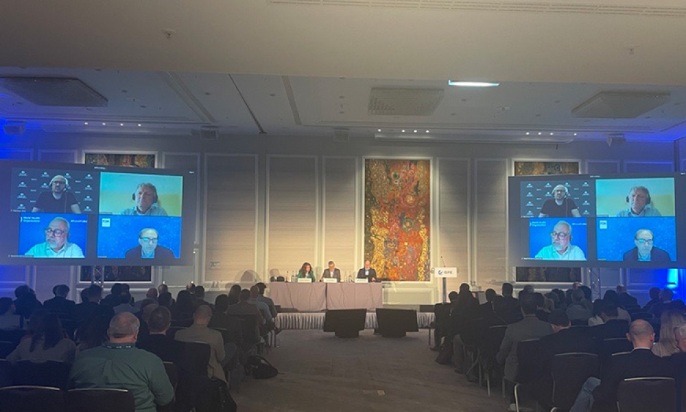
On 13 March 2024, ISPE concluded the 2024 Aseptic Conference with a regulatory panel question and answer session. Attendees were invited to submit questions to representatives from the Austrian Agency for Health and Food Safety (AGES), US Food and Drug Administration (FDA), Regierungspraesidium Tübingen (RP Tübingen), World Health Organization (WHO), Therapeutic Goods Administration (TGA), and...

The pharmaceutical industry stands at the precipice of a revolution as emerging digital technologies provide new opportunities to boost productivity through continuous process improvements. The Pharma 4.0™ framework, an adaptation of the broader Industry 4.0 movement, aims to transform how drugs are produced and delivered.

With the approval of the first gene edited therapeutic in 2023, production of gene edited therapies is accelerating, introducing tough decisions for manufacturing development. Gene editing therapy production is complex, often involving multi-modality manufacturing operations in one facility to produce a single therapeutic. This article considers whether retrofitting an aging monoclonal...


Currently, there is no single guidance document providing a comprehensive roadmap for executing digital validation. While elements from ISPE GAMP® Guides Series and the ISPE Baseline® Guide: Volume 8 – Pharma 4.0™, apply to digital validation, there is no consolidated resource addressing common questions. The authors of this Concept Paper therefore advocate for the development of a Good...

A set of principles to be considered in the journey to adopting and deploying an architecture capable of supporting Pharma 4.0 Plug & Produce capability.

Explore June’s top reads in Pharmaceutical Engineering®—from cleanroom pressure design and AI validation to modular cell therapy manufacturing and ATMP access. Discover strategies for resilience, sustainability, and speed in pharma facility innovation.


The new ISPE GAMP® Guide: Artificial Intelligence provides a comprehensive, state-of-the-art best practice framework to efficiently and effectively achieve high-quality AI-enabled computerized systems in regulated life science areas. It bridges established GAMP concepts with...

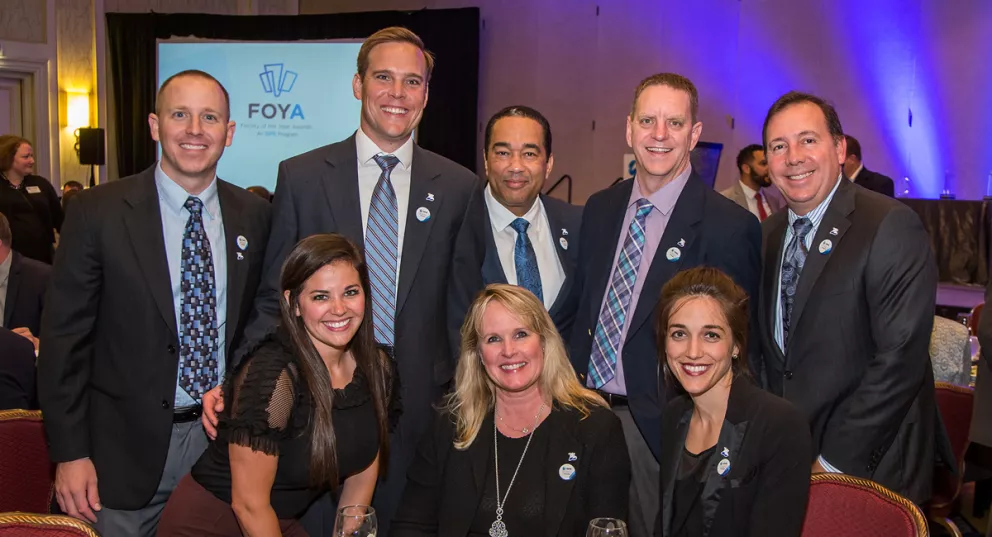
Each year, FOYA showcases innovation, excellence, and progress in the pharmaceutical industry. The winners exemplify state-of-the-art design, cutting-edge technology, and industry best practices, continually setting new standards for what constitutes a winning project. This constant evolution keeps FOYA fresh and original, making it all the more remarkable that FOYA is celebrating its 20th...

The pharmaceutical industry is experiencing a pivotal transformation. As professionals strive to develop therapies faster, more cost-effectively, and with greater precision, Pharma 4.0™ emerges as a powerful framework for change. This evolution is not only technological—it is cultural. It challenges organizations to become more agile, data-driven, and patient-focused.


The pharmaceutical industry is under increasing pressure to develop new therapies at a faster pace, while lowering drug costs, enhancing quality, and maintaining safety and a robust supply chain. Validation 4.0 ensures that validation processes are not a bottleneck but a strategic enabler of innovation, quality, and compliance by embracing artificial intelligence (AI), Internet of Things...

As the pharmaceutical industry evolves, sustainability is becoming a key driver of operational efficiency and long-term success. From reducing carbon emissions to enhancing workforce safety, companies are aligning their practices with sustainability goals. The 2025 ISPE Annual Meeting & Expo is the ideal platform to exchange ideas and...

The pharmaceutical industry is no stranger to innovation. From pioneering drug development to advanced manufacturing processes, it thrives on new ideas. But when it comes to construction, particularly the delivery of critical infrastructure such as laboratories, cleanrooms, and research facilities, many companies in the sector still rely on traditional building methods.


The pharmaceutical sector is undergoing a profound transformation. As digital technologies continue to evolve, organizations are under increasing pressure to modernize legacy systems, enhance operational efficiency, and maintain compliance in a rapidly shifting regulatory landscape. The Digital Transformation track at the

Each issue of Pharmaceutical Engineering® covers a wide range of topics relevant to the pharmaceutical industry, including scientific, technological, and regulatory advancements throughout the entire...

On the closing morning of the 2025 ISPE Europe Annual Conference, Ian Jackson, an expert GMP inspector with the Medicines and Healthcare products Regulatory Agency (MHRA), presented MHRA’s Policy for the Future and Globalized Industry.


At the 2025 ISPE Europe Annual Conference held 12-14 May 2025 in London, the European Medicines Agency (EMA)’s Head of Quality and Safety of Medicines Department, Evdokia Korakianiti, highlighted the many...


In a world defined by rapid scientific progress and evolving market demands, the ability to adapt, innovate, and sustain excellence is no longer optional—it’s essential. The 2025 ISPE Biotechnology Conference,...
Sponsored content is the sole responsibility of the authors and is not endorsed, reviewed, nor a published article of Pharmaceutical Engineering® magazine or ISPE.

When you’re in the pharmaceutical industry, you’re going to be audited — are you ready? Authored by Kneat’s audit expert, Joe Azzarella, Audit Preparedness: Using Digital Validation to Be Ready for Anything, explains what you should expect before, during, and after an inspection and what you can be doing to make sure you pass with flying colors.

In the rapidly evolving pharmaceutical landscape, manufacturers face mounting pressure to deliver safe, effective drugs swiftly while navigating complex regulatory and operational challenges. This eBook explores how digital transformation is reshaping pharmaceutical manufacturing by accelerating time-to-market, enhancing facility performance, and driving sustainability. It outlines strategic...

In an industry where reliability, compliance, and efficiency are non-negotiable, how mature is your approach to asset management? The Roadmap to Asset Performance Management in Life Sciences provides insights on how leading companies are transforming their maintenance strategies into strategic drivers of business performance.

Validation professionals are under pressure — from rising workloads to new regulatory demands. Backed by four years of industry data, this year’s State of Validation report — authored by leading life sciences market research Jonathan Kay — reveals how organizations are tackling challenges like audit readiness, resourcing constraints, and the shift to digital systems. Discover benchmarks, best...

In the world of pharmaceutical and life sciences manufacturing, purity, reliability, and performance are non-negotiable. That’s why engineers and facility managers are turning to SYGEF® PVDF piping systems from GF Piping Systems—a solution engineered to meet the most stringent demands of high-purity applications.

Whether networking at events or collaborating through our Communities of Practice, the value of an ISPE membership is in the connections made between pharmaceutical industry professionals and Regulators to collaborate on solutions to common goals and challenges.
Are you a subject-matter expert in the global pharmaceutical industry? Are you brimming with knowledge about the latest technical developments or regulatory initiatives? Have you found an innovative solution to a real-world challenge?
Contribute your knowledge and experience to the always-evolving pharmaceutical industry!
Do you know someone whose profile or work should be featured in Pharmaceutical Engineering? Contact ISPE Publications Department.