Artificial Intelligence Used to Optimize Fluid Bed Drying

The main benefits realized from this project: Best control of product quality by means of an increased process knowledge as per International Council for Harmonisation of Technical Requirements for Pharmaceuticals for Human Use (ICH) Harmonised Tripartite Guideline Q10: Pharmaceutical Quality System expectations; process time reduction and increase of machine availability; friendly-environment initiatives by reducing atmospheric emissions and lowering power consumption (energy savings);applicability of the digital twins concept allowing studies and forecast of multiple “what if” scenarios for optimal solutions; and other positive side effects such as enabling multivariate statistical process control, facilitating the implementation of continuous process verification, reducing time, and increasing effectiveness of investigations for quality events.

Background

Manufacturing Process

The manufacturing process of an oral-tablet bulk drug product is divided into several phases, such as weighing/dispensing, sizing, blending, granulation, drying, sieving, tableting, and coating.1 This article focuses on the drying process, specifically fluid bed drying technology.2 Fluid bed drying is commonly used in pharmaceutical manufacturing because it is more efficient for drying granules contained in wet granulation. The granules are dried by the combination of the diffusion of moisture from the solid, mediated by hot air, and the entrainment of this moisture by forced convection. In this operation, the granule must be uniformly fluidized by hot air and dehumidified so that an efficient transfer of mass and energy takes place. The higher the temperature and the higher the intake air flow, the shorter the drying time. The inlet air temperature, which must not exceed the critical temperature of the product (pharmaceutical stability), is modulated by the temperature signal, which is indirectly measured by the sensor in contact with the air outlet.

The drying process in a fluid bed machine consists of three phases: preheating, drying, and cooling. Preheating is performed without the product and is intended to minimize the overall process time by ensuring that the energy involved in the next step will be used to heat the product and evaporate water instead of heating the stainless steel of the equipment. Drying the product is when the water evaporation takes place. Once the product drying is finished, the equipment cooling begins; this ensures there is no water condensation on the dried product if it is taken out of the drier while still hot.

Each of these phases involves a cost: the use of the machine, the efforts of the operator, the cost of the energy required to heat and move the air. This article covers the preheating and drying steps with specific approaches for each, leading to two different modeling exercises.

Equipment: Fluid Bed Dryer

We used a fluid bed dryer with standard sensors to allow for suitable control of the process parameters. The airflow, air pressure, and temperature of the incoming filtered dry air, and up to 56 other variables, are monitored and recorded in real time. Equipment setup is automatically driven by product receipts with the exception of steps that operators control manually (based on operator experience and batch-to-batch analytical results) before ending the process. The process duration is strongly linked to the operator experience.

• 1Anderson, S. Making Medicines: A Brief History of Pharmacy and Pharmaceuticals. 2005: Pharmaceutical Press.
• 2Dufour, P. “Control Engineering in Drying Technology: Review and Trends.” Drying Technology 24, no. 7 (2006): 889–904. https://doi.org/10.1080/07373930600734075

Data Process

Figure 1 shows the supervisory control and data acquisition (SCADA) panel3 used by the operators to interact with the machine in real time; they can start and stop the controller and monitor the inlet air temperature and flow indicators. The sensors from the SCADA panel measure continuously and create minute-long time-series data points, one for each of the parameters. We used data from a period spanning 1.5 years, which have been exported into a table with more than 700,000 rows and 56 columns. Due to the high volume of data (more than 3 GB of data), we have selected an appropriate standard platform and its advanced analytics module, using Python for data analysis.

The data were cleaned: duplicates of time stamps and empty data cells were removed.

Our studies are based on examining individual drying processes consisting of preheating, drying, and cooling, called lots or batch here. Individual lots can be identified in the SCADA time-series data points by looking into the difference between the dryer inlet and outlet air temperature.

• 3Da Silva, C. A. M., J. J. Butzge, M. Nitz, O. P. Taranto. “Monitoring and Control of Coating and Granulation Processes in Fluidized Beds: A Review.” Advanced Powder Technology 25, no. 1 (2014): 195–210.

AI Approaches

In our study, we used two different approaches to meet the goals highlighted in the introduction.4 ^,5 The first approach focuses on methods to show the potential to reduce preheating and drying times using endpoint prediction, and the second approach focuses on using a digital twin to simulate the process with modified configurations in order to find the best setup.

Endpoint Prediction Study

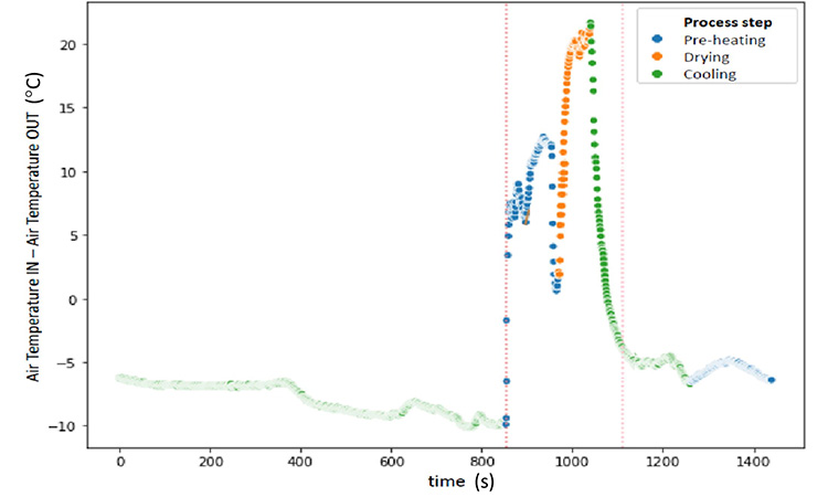
During this process step, the wet granule is not uploaded yet. The supplied energy is used to heat the empty equipment. Once the stainless steel reaches the targeted temperature, the equipment remains at a stable temperature awaiting the next step (drying of loaded product). Any extension of this time causes energy consumption without positive contribution to quality or process duration.

The model used to identify the step endpoint is based on forecasting the step duration by predicting the minimum difference between IN and OUT temperatures when the equipment reaches stability. Thus, the optimal endpoint for the preheating phase is calculated as the forecasted function derivative=0 and the linked time is given as the outcome of the algorithm.

Preheating modeling results

Due to the proportion between rows and columns in the training data, dimensionality reduction techniques are used to minimize the number of features. Data normalization and principal components analysis (PCA).6 were used, with the model being based on PCA and multiple linear regression.

The metric for evaluating the models is R2 (determination coefficient), which conveys the percentage of the variance explained by the model. The trained model reached R2=0.88 and showed appropriate predictions with equal R2 on the 25% of data reserved for validation purposes.

Time reduction targeted a significant reduction of 37 minutes per batch, leading to an increased equipment availability of 24% and energy savings of 4000 KWh per year (90 batches/year with an average reduction of 45 kWh/batch from the preheating step).

Drying modeling results

The same process was applied to the preheating phase. The combined results are summarized in Table 1.

In addition to these savings, there are process gains in duration stability and a significant reduction in variability of the results when comparing the production before and after the AI algorithm implementation.

Digital Twin Study

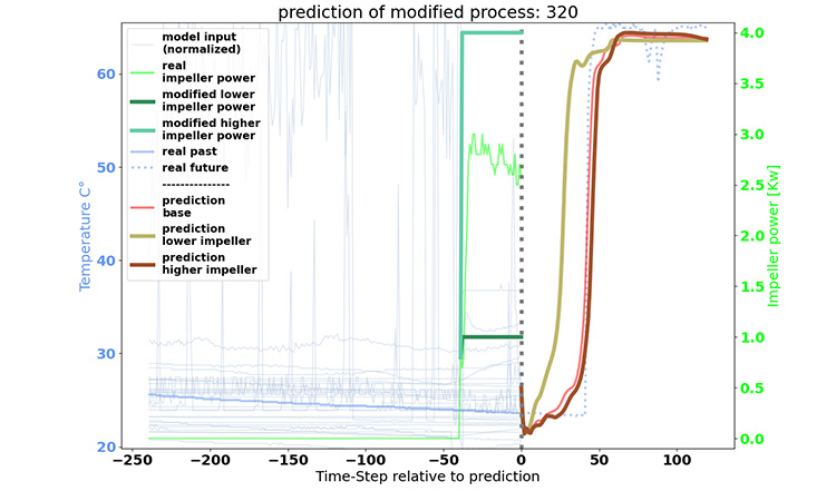
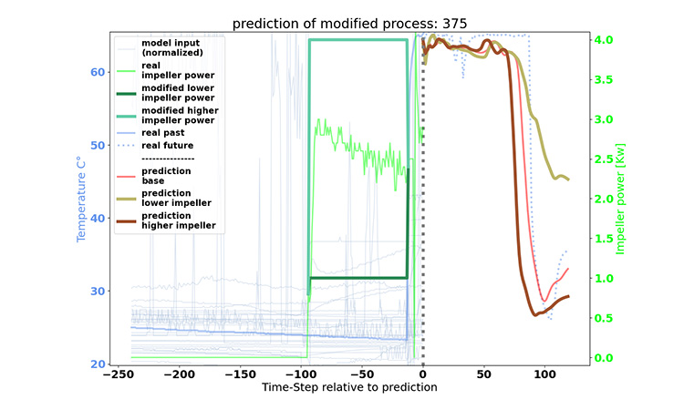
In our second approach, we enabled simulations of the drying process digitally on the computer. A neural network was trained and fed with input parameters measured with the sensors of the fluid bed dryer to predict the evolution of the drying process. In this exercise, we use the neural network model built to predict the behavior using new values on input parameters. This will enable us to conduct cheap and easy testing with the computer instead of producing costly experiments in real life.

In other words, we generated a virtual representation of the drying process for studies in the digital world, which can provide feedback to the real drying process. Such concepts have become known as “digital twins” in recent years,7 ^,8 a term we want to adopt here.

For the digital twin, we need an algorithm capable of processing time-series data, i.e., a multitude of time-series data points as input data, and a few time-series data points as output data. One of the few algorithms that can do this are recurrent neural networks, or, more specifically, long-short term memory neural networks (LSTM).

An LSTM is generated by predefining an architecture of functions that process a certain input in order to relate it to a certain output. Each of the functions contain weights that, in an iterative process, are configured in a way to optimally transfer the input to its associated output. By doing so, we imply that the model learns all the relations and interactions between the set of input parameters and their response and is capable of representing them in a formal mathematical way. This learning process is called model training and is done on large amounts of historical data.

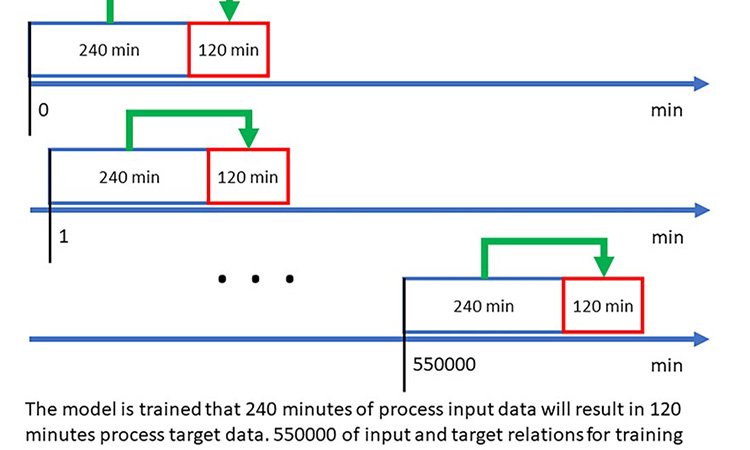
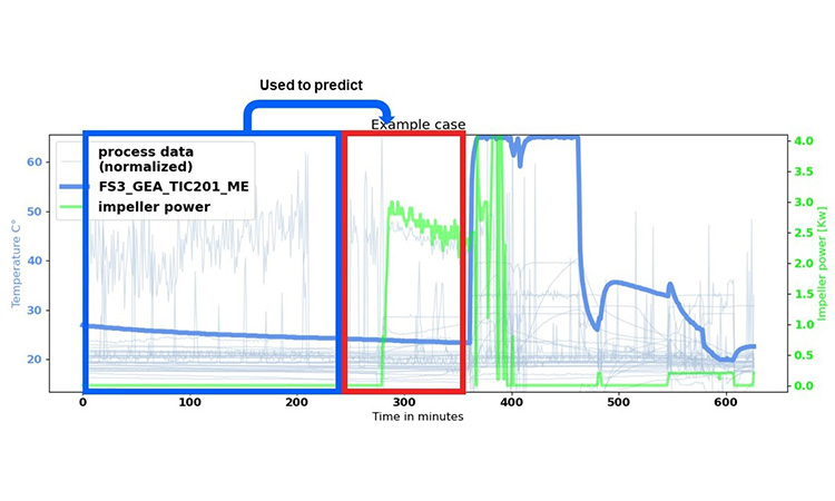
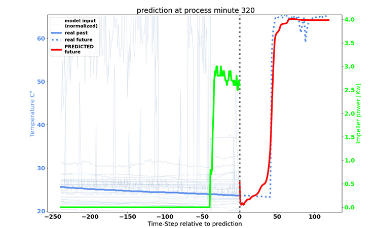
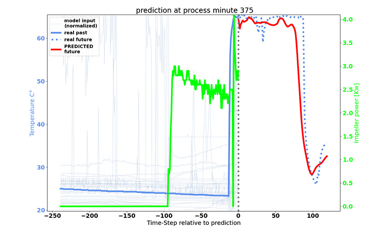
In our example, we wanted to shorten the drying duration to increase machine availability by finding an optimal LSTM configuration. The time-series data of the fluid bed dryer served as the input parameters for the model. For the output, or the target, we chose the parameter airflow temperature. The model response for this curve allows us to determine the drying duration.

The model is trained that 240 minutes of process input data will result in 120 minutes of process target data. As depicted in Figure 3, 550,000 minutes of input and target relations for training are created by starting at minute 0 and increasing by 1 minute.

• 4Buvailo, A. “The Why, How and When of AI in the Pharmaceutical Industry.” Forbes. Published 24 April 2018. https://www.forbes.com/sites/forbestechcouncil/2018/04/24/the-why-how-and-when-of-ai-in-the-pharmaceutical-industry/?sh=4958370d6d07
• 5Markarian, J. “The Internet of Things for Pharmaceutical Manufacturing.” PharmTech. Published 2 September 2016. https://www.pharmtech.com/view/internet-things-pharmaceutical-manufacturing
• 6Hotelling, H. “Relations Between Two Sets of Variates.” Biometrika 28, no. 3/4 (1936): 321–377. https://doi.org/10.2307/2333955
• 7Negri, E., L. Fumagalli, M. Macchi. “A Review of the Roles of Digital Twin in CPS-based Production Systems.” Procedia Manufacturing 11 (2017): 939-948.
• 8Rosen, R., G. von Wichert, G. Lo, K. D. Bettenhausen. “About the Importance of Autonomy and Digital Twins for the Future of Manufacturing.” IFAC–PapersOnLine 48, no. 3 (2015): 567-572. https://doi.org/10.1016/j.ifacol.2015.06.141

Our model architecture consists of two layers, each of them containing 100 neurons. We used the Adam optimizer and the Huber loss function. We developed the model using Python with the keras and tensorflow libraries.

The aim of this model is to test its sensitivity in response to changes in the input data and not for prediction purposes, so it does not require good predictions, but we need a case in which the model replicates the relations between the set of input parameters and its target. This can be done more accurately if the original response is already known to the model. We further argue that modifying the input data results in new data that the model has not seen before during the training; we assume the new data is independent from the training.

Example using observed input

We now look closer into one instance of a drying process, to which we want to apply our digital twin to conduct a sensitivity study.

Figure 4 shows a whole drying process including 350 minutes before its start. At around minute 280, the impeller is turned on with values around 3 -2 kW, and about an hour later, the drying starts as indicated by a steep increase of the airflow temperature.

To begin, we provide the model with the airflow temperature data in the blue box and expect to receive the values in the red box as a response (target). The curve of the impeller power is shown in green, and the time series of the 30 other input parameters are in thin grey [unitless].

Figure 5 shows where the model response very closely matches the observations of the airflow temperature. We move the two boxes onward in time, minute by minute, and get the same results as demonstrated below until the start of the drying moves into the red box.

In the left-hand side of the dashed vertical line, all of the data input that enters the model with airflow temperature is in blue and impeller power is in green. In the right-hand side of the dashed vertical line, the model response (predicted temperature) is in red and their observed values are in dashed blue.

An example of the model response is shown in Figure 6, where the steep changes of the airflow temperature are visible very accurately in the model response in time and extent.

Moving forward in time, the same holds for the end of drying in Figure 7, which again is very accurate in the model response.

Example using modified input

In the previous example, we saw that our digital twin fares well in the base experiment replicating the observations. With this in mind, we apply our digital twin to learn what happens if we run the same drying process with a modified impeller power as input parameter. Therefore, we undertake the same experiment and feed the model with the same input data, but we lower the impeller power and lower its values from around 3 kW down to 1 kW and study the model response.

The response for the start and end are shown as light brown lines in Figures 8 and 9. The drying is projected to begin earlier, at around 10 minutes, but to end later, closer to 20 minutes, as indicated by the drop of the airflow temperature curve. In addition, the dropping is not as pronounced as in the real curve within this time window. We conclude that lowering the impeller power before drying extends the drying period by about 20-30 minutes.

In Figure 8, one version shows values lowered to 1kW (dashed green line) and one with values lifted to 4kW (dash-dotted green line). In addition the model responses are shown for the base input (red line) and for the modified input with lower (dashed orange) and lifted (dashed-dotted yellow) impeller power.

Next, we feed the model with increased impeller power to up to 4kW as shown as dark brownish line (sienna) in Figures 8 and 9. The drying is projected to start a bit later compared to the base experiment power, and to finish earlier, closer to 10 minutes. Also the minimum of the airflow temperature curve is lower than in the base experiment. Hence we conclude that increasing the impeller power before the drying reduces the drying time.

Lower/higher impeller power means less/more air and thus less/more energy is entering the process before it starts. From a physical and/or galenical point of view, the model response is consistent because less/more energy provided to the system means lower/higher evaporation rates, which themselves potentially extend/shorten the drying.

Another or additional explanation could be the impeller’s impact on the granule size. Lower/higher impeller power may generate bigger/smaller granules for the drying, and smaller granules may favor a quicker drying.

Conclusions

The first model approach (endpoint prediction using temp IN versus temp OUT as response of the PCA + linear regression) found the potential for significant reductions of duration and energy keeping the state of control of the process. For either preheating or drying, the following outcomes were reached:

• Yearly energy savings of 5.5 MWh for a production of 90 batches/year
• Higher process stability in terms of duration and moisture results
• Increase of equipment availability

The second model approach shows how to apply the digital twins concept to our drying process and enables sensitivity studies in the virtual world. One application could be trial runs that are conducted to find the most suitable configuration before setting up the actual production process. Each of these trial runs can be costly, but transferring some of these trial runs into the virtual world would not only save a lot of money, but would also allow for many more trial runs and thus more robust results.

Another application could be during production, with the digital twin suggesting optimal parameter settings to the operator. If, for instance, sensitivity studies were triggered before switching on the impeller, an optimal setting could be determined right before starting the drying. This setting would not only be based on the static specifications defined for the process, but considering the most up-to-date measurements from the sensors could react to any incidents happening on the machine. In this context digital twins can become even more valuable, because the model is not only capable of analyzing one parameter, but a multitude of parameters and their interactions at the same time.