Sampling Considerations in Continuous Manufacturing

Sampling is the selection of a representative portion of the population to make inferences about the entire population. In pharmaceutical manufacturing, samples are drawn from different stages of the process for both controlling process parameters and assessing drug product quality. In the case of a traditional batch process, a fixed amount of material is processed and the batch quality is established after it has been fully manufactured. In contrast, in a continuous manufacturing (CM) process, material is continuously flowing through the process from one unit operation to the next, being converted from raw materials to finished product, and the control strategy focuses on maintaining a state of control of the process (after its start-up and before its shutdown) as raw materials continuously enter the process, so that good quality product is produced. This article describes aspects of sampling within a continuous process during both development and commercial manufacturing of solid oral dosages and draws comparisons to sampling in the traditional batch process.
Sampling Data Sources for Continuous Manufacturing
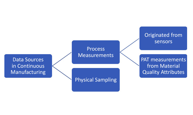
Data sources represent mechanisms for extracting sampling information from the CM process for inferential purposes. As summarized in Figure 1, these mechanisms can be generally separated into two categories: physical sampling and process measurements. Sampling by physical removal of material for off-line or at-line analytical testing is employed in both traditional batch processes and CM. In this article, the term “physical sample” will be used when referring to removal of material from the line.
Two types of process measurements could be considered for CM, both originating from process analytical technology (PAT). 1 The first originates from sensors measuring the performance attributes of the process itself. The second encompasses PAT measuring raw or in-process material quality attributes and translating these raw measurements into the attributes in question; the translation is frequently based on multivariate models applied to near-infrared (NIR) spectroscopy signals. Note that the models must be developed and calibrated against laboratory-analyzed physical samples.
- 1US Food and Drug Administration. “Guidance for Industry: PAT—A Framework for Innovative Pharmaceutical Development, Manufacturing, and Quality Assurance.” September 2004. https://www.fda.gov/downloads/drugs/guidances/ucm070305.pdf
All these information sources (physical samples, online material measurements, and process measurements) play a role in the development of process understanding. And, as process knowledge matures, strategic decisions can be made as to which elements are required to ensure material quality as well as appropriate limits for the respective measurements.
As is the case with batch processes, the objectives for physical sampling and especially PAT measurements change substantially as the product moves through development toward commercial production. The use of NIR methods requires model development that translates spectroscopic signals into a response of interest (e.g., concentration of active pharmaceutical ingredient). Hence, during early product and process development, measurements must be gathered from both NIR and traditional at-line or offline analytical methods to define and refine the prediction model. In this early stage, final quality statements should be based on the results of physical samples. Before such a model is formally validated, the data collected from PAT cannot be used for absolute quality statements about the final product for purpose of release. However, nonvalidated PAT measurements may still provide an indication of quality and potentially be used as supportive information. Nevertheless, until PAT models are fully developed, PAT data collection and physical material sampling should be aligned so that collected data can be used for PAT model development and for quantifying the model’s accuracy and precision.
As the process approaches validation, both physical sampling and PAT should continue to be used. Physical sampling and validated PAT measurements allow quality statements to be made of the final product, with PAT enabling the monitoring of the quality attributes throughout the continuous run. Real-time release testing (RTRT) strategies may be employed to further replace certain physical sampling–based testing with validated PAT measurements. In general, both data sources should be leveraged to confirm process quality and enhance process understanding until all processes and methods are appropriately validated.
Both the physical sizes of the sample and the physical sample representation of all manufactured items play a role in determining the representativeness of inline PAT measurements about the entire process. 2 The material flowing through a continuous line is not truly observed continuously; instead, the measurements are taken at a certain frequency, and each measurement represents some fractional amount of material out of the total. The minimum frequency is determined by the residence time distribution (RTD)—a distribution of the time it takes for a distortion to propagate throughout the line (or part of the line, depending on the presence/location of diversion points within the process). Variability in feed rates is attenuated by the blenders and mixing in a tablet press feed frame or encapsulator bowl, and the resulting blend uniformity may be quite insensitive to short-time feeder flow distortion. The combination of RTD studies with quality requirements allows determination of the minimum required measurement frequency. Generally, the maximum frequency of PAT measurements is bounded by the device capabilities. Once the PAT measurement frequency is determined, a quantitative estimate of the variability of the “unseen” material is established to provide confirmatory statements of the acceptability of the sampling frequency.
The precise location of the PAT sensor is especially important in relation to the point of physical sampling. Because of the dynamic nature of a continuous line and material transport, blend uniformity measured between two-unit operations may change. For example, because additional blending of material occurs during transportation, a sensor installed at the output of the mixer may provide different blend uniformity results when compared with a sensor on the feed frame of a tablet press.
During process validation, it is vital to collect sufficient evidence to confirm that process performance is satisfactory when the process is run as designed and to ensure that physical sample measurements confirm performance as indicated by online measurements. Commercial production is considered satisfactory unless confirmatory measurements suggest otherwise. Once validated, the role of the physical sample measurements changes from being the primary indicator of quality to solely confirming quality, because quality is ensured by the process parameters staying within acceptable ranges. Indeed, for many processes, the PAT measurements become confirmatory as well, providing evidence that the process is performing acceptably. The difference between the confirmatory physical samples and confirmatory PAT measurements is that the PAT measurements provide a high-frequency signal of process quality that depends on a predictive calibration model, whereas the physical samples provide a low-frequency quality signal using reference methods. PAT measurements generally provide a low-cost input to a statistical control check against special-cause process upsets.3
In addition to PAT measurements being used to monitor process quality, they may also be incorporated into a feedback loop to further reduce variability about a desired quality target. Upstream process settings may be adjusted based on the downstream PAT measurement. If the PAT is intended to be used in a feedback capacity or as part of the control strategy of a validated process, the PAT measurement becomes a required process element and should not be eliminated (unless there is another suitable analytical method available). This is true even if historical performance shows that the process is well behaved without the collection of PAT measures during process quality monitoring. In contrast, when not operated in a feedback loop, certain PAT measurements of material quality attributes may be unnecessary if a strong relationship between these material quality measurements and other associated process measurements is sufficiently demonstrated.
Sampling Frequency Assessment Strategies
Within the traditional batch manufacturing approach, quality is typically ensured by maintaining process parameters within certain predefined boundaries and then confirming the quality of the product produced through postproduction testing. A key aspect of this batch manufacturing approach hinges on establishing the quality of the batch after it has been fully manufactured. This is in juxtaposition to the CM process, where material moves through the process from one unit operation to the next, being converted from raw materials to finished product. Best practices involve a continuous control strategy that focuses on establishing the process is in a state of control at the time that good product is being produced. In other words, batch manufacturing focuses on demonstrating the quality of the product within space, whereas CM focuses on demonstrating the quality of the product in time.
- 2US Food and Drug Administration. “Development and Submission of Near Infrared Analytical Procedures: Draft Guidance.” March 2015. https://www.fda.gov/downloads/Drugs/GuidanceComplianceRegulatoryInformation/Guidances/UCM440247.pdf
- 3Box, G. E. P., and A. Luceño. Statistical Control by Monitoring and Feedback Adjustment. Hoboken, NJ: Wiley & Sons, 1997.
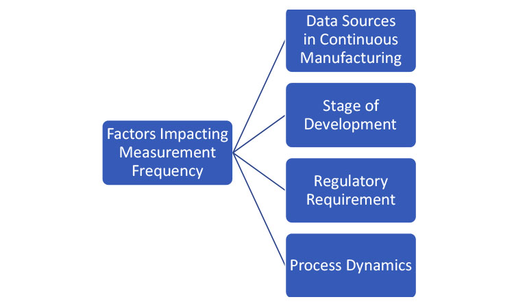
To determine the frequency of obtaining the product- or process-related quality attributes, one must consider the data source, the stage of development (as discussed in the previous section), and the purpose of the data. Figure 2 lists some of the factors that affect the measurement frequency. The collection of process and product data can be generally organized into two categories: data that are used for active control of the process and data that are used for confirmation that the process is operating as designed.
If the data are being collected to make control decisions within the process, the collection frequency should be driven by the dynamics of the process. Process dynamics is the understanding of how a process changes in time. When a disturbance happens within a process, the time it takes for the disturbance to propagate through the process is known as the process’s characteristic time (i.e., the RTD). If data are being used for control, the collection frequency must be fast enough to provide a measurement of the process attributes that has adequate statistical power to determine the appropriate control output. If the data are being used for confirmation, the collection frequency should be driven by the time it takes to produce the batch (this is much like the batch manufacturing approach).
As noted previously, data sources can be generally separated into two categories: process measurements and physical sampling. Process measurements are typically high-frequency measurements, which typically repeat on the scale from milliseconds to tens of seconds. They are normally nondestructive, and they can be performed either online (a sensor looking at part of a stream) or inline (the entire process stream passing through a sensor) or come from sensors integrated within the process equipment (e.g., compression force measurement within a tablet press). Process measurements are usually automated and require minimal or no operator interaction. Physical sampling involves collecting material samples from the process stream and submitting them to testing away from the line. The collected samples can be analyzed at the line, where the analysis is carried out near the process, or taken to a lab for traditional wet chemical analysis. Physical sampling approaches are often at least somewhat operator-driven activities. They are frequently, but not always, destructive and results can take minutes to weeks to receive.
There is a natural synergy between the high-frequency demands of the data needed for control and the high-frequency capabilities of process measurement. Likewise, the low-frequency capability of physical sampling makes it an appropriate option for confirmatory testing. While this heuristic is generally reliable, special cases do apply. For example, the high-frequency nature of a process measurement would not preclude its use as a confirmation test. Likewise, if a physical sampling approach can be used to provide feedback information more quickly than the characteristic time, it would be suitable for control. The key concept is that the frequency of each test must be defined with respect to the purpose for conducting the test.
As defined in ICH Q10, state of control is “a condition in which the set of controls consistently provides assurance of continued process performance and product quality”. 4 Consequently, a process can be said to be in control when the critical quality attributes are demonstrated to be within predefined levels by the data collected from the process via process measurement, physical sampling, previously established process capability, or some combination of these. Several common examples of quality attributes and control strategies will be offered to provide context to the discussion.
The simplest way to demonstrate a particular quality attribute is within range is to directly measure it (assuming that is possible). For example, encapsulators are often paired with check-weighers to individually assess the weight of each capsule in the product stream.
While direct measurement is ideal, it is not possible for most quality attributes. For example, consider the weight of a tablet. While tablet presses use a force control loop to monitor and adjust the amount of volume to fill in the die, the force loop does not directly measure the tablet weight; instead, it is a process measurement that correlates with the weight. The force measurement can be used to make an individual quality statement about each tablet compressed, predict the variability of the product stream, and segregate individual tablets from the stream. However, the force loop by itself cannot predict the actual tablet weight. The latter is enabled by externally assessing the tablet weight and adjusting the press to keep the tablet weight on target. This well-known feedback loop is an excellent example of combining a high-frequency process measurement with a low-frequency sampling-based measurement to ensure a process stays in a state of control and assures product quality.
Of course, the actual final critical quality attribute of a tablet or capsule is not its weight; it is the dose, which is the product of the concentration of the API within the drug form and the aforementioned weight. Within the CM paradigm, there are two common options for assessing the concentration of the blend: (a) prediction of the concentration using loss-in-weight feeder data combined with a dynamic process model, or (b) prediction of the concentration using a spectrometer (e.g., NIR or Raman) and an associated multivariate model to assess the concentration. In both cases, it is typical for the predictions of the concentration to be capable of capturing the average concentration of the process stream, but not necessarily the variation in the process stream. The multivariate spectrometer variation is often driven by noise associated with the instrument and the way the sample is presented to the sensor. The feeder data approach is typically based on a perfect mixing model, which does not account for the level of micromixing within the process. The most common approach for addressing the variability of the stream is to use development trials to demonstrate the extent of natural variation within the process stream. If the variation is found to be small compared to the specification limit, targeting and adjusting ensure that the mean concentration is tightly controlled within a specified control limit; this is a perfectly acceptable control strategy.
For batch release of a final product, the physical sampling frequency will need to be aligned with regulatory requirements. For traditional batch testing, the number of representative physical samples for release will be smaller than the number of measurements when using PAT. However, in both instances, the number of samples and associated acceptance criteria should provide acceptable assurance of the product’s ability to meet the specifications.
Results of high-frequency data streams should be interpreted within the context of the capability of the method and the known behavior of the process, including the extent to which the measurements could be considered independent and identically distributed. High-frequency data streams will lead to occasional outlying observations. For example, consider a multivariate spectroscopic process measurement such as a NIR method. Assume that this method is developed to monitor the average concentration of the process, and the probe frequency is orders of magnitude higher than the characteristic time. A few outlying measurements can be safely ignored because it has been previously established that the stream does not vary appreciably in such a short time frame. Therefore, these variations are likely caused by variation of the method and not the process. Similarly, a single missing observation in the case of multivariate spectroscopic (or other) method does not necessarily raise immediate concerns about product quality.
Next, consider an extreme compression force measurement within the tablet compression scenario discussed previously. This is a measurement of an individual tablet being created and is indicative of a single out-of-specification unit. The proper response would be to reject that unit because under- or overfill events can occur.
Establishing that a process is operating in a controlled state is key to the successful implementation of CM. The need to demonstrate the control within a time frame that is relevant to the process (e.g., the characteristic time) calls for a more nuanced discussion of what data are collected from the process and how they are used. For most continuous processes, the resulting control strategies will be a combination of many of the tools used within the traditional batch paradigm (e.g., in-process controls and stratified sampling), but they will be built around advanced high-frequency data streams that can help demonstrate and maintain a state of control.
Control Techniques and Diversion and Redundancy Decisions
Physical samples may be gathered throughout a batch to con rm that the process is producing or has produced products or intermediates (e.g., blends or uncoated tablets) with quality characteristics within the prespecified attribute ranges. These confirmatory samples provide some assurance that the process is operating or has operated as desired. Generally, these physical samples are low frequency and are used to augment other process or inline measurements that generally provide a higher-frequency assessment of process performance. For example, feeder rates and spectroscopic signals of the blend at the feed rate ensure consistent blend proportions, torques on the mixer ensure consistent flow of powders, and compression forces ensure consistent tablet weights. These high-frequency product and process measurements could be collected as often as every few fractions of a second and could thus provide thousands of measurements per hour of a batch.
From a volume perspective, the high-frequency process sensors and inline measures overwhelm the low-frequency sample measurements, and the value of the physical sample measurements is limited. However, the physical sample measurements have two potential advantages. First, they are generally collected from final or near-final products (e.g., uncoated tablets) and thus reflect the totality of the process, including any atypical behavior that may affect quality. Second, they use reference methods for measurement. On the other hand, the critical disadvantage of physical samples is that because of their low sample frequency, they may miss short-term changes in the process.
Inline measurements near the end of the process combined with well-developed predictive calibration models allow accurate and precise estimation of reference method measurements and can match the two advantages of physical sample measurements. For example, a well-characterized spectroscopic model that translates measurements of the blend at the feed frame into concentration measurements can be used in combination with a compression force gage at the tableting station that provides indirect tablet weight measurements, and this combination can provide tablet potency estimates that accurately reflect the behavior upstream of the feed frame. These potency estimates are thus valid surrogates for reference potency measurements. In such a situation, the confirmatory aspect of physical sample potency measurements is redundant and can potentially be replaced by this indirect method, if it is appropriately validated. Also, relative to infrequently gathered physical measurements, the high-frequency measurements can be configured to have a high probability of detecting shortterm aberrations in the process. 3
Well-designed control systems incorporate combinations of sensors and inline measures that span the process and either prevent quality aberrations or detect their existence. For example, mass flow sensors can ensure that the correct proportions of powders are fed to a mixer. However, if two excipients were inadvertently loaded into the wrong hoppers, the individual feeders may lead to normal mass flows (of the switched materials); the mass flow sensors would not detect this error, but a NIR signal at the feed frame could provide evidence of the mistake (e.g., through extreme Q residuals, which measure the difference between a sample and its projection into the principal components from a model 5 ).
Equipment design may also minimize the likelihood of potential failure modes. For example, the path of powder movement may be designed to eliminate ledges that allow powder aggregation and to be as short as feasible.
Typically, the control system design incorporates failure modes and effects analysis combined with verification testing during development to prove that untoward changes are detected. The control algorithms generally incorporate warning and alarm limits that signal or stop the process when atypical readings are obtained. When the control system design has been proven to effectively prevent or detect product quality issues, the need for confirmatory samples is obviated.
Both univariate statistical process control (SPC) and multivariate statistical process control (MSPC) may be used to evaluate current performance relative to past performance and could provide assurance that the process is performing within historical norms. Signals (atypical measurements or patterns of nonrandom behavior) may trigger process stoppages to allow investigation or diversion of material to prevent questionable product from being forward-processed. In cases where measurements are affected by autocorrelation, the use of SPC and MSPC techniques could result in an increased number of false alarms 6 and the use of timeseries techniques should be considered. 7
When an end or near-end-of-process measurement of a quality attribute is unavailable, the process should be evaluated to determine whether upstream and correlated downstream measures provide acceptable assurance of quality without confirmatory physical sample measurements. Past process behavior and equipment design will influence this assessment. For example, content uniformity in a continuous direct compression tablet process is largely determined by feeding powders at the targeted rate, providing adequate mixing, and compressing the desired amount of blend into tablets. As mentioned previously, sensors on each feeder, the mixer, and the compression station can provide acceptable evidence of consistent potency.
In some cases, physical sampling will be deemed necessary to verify that the process has not experienced a special-cause event. During development, experiments can be conducted to quantify the impact of certain special causes. For example, drug substance feed rates of various magnitudes and durations can be enacted, monitored, and modeled to provide an understanding of the powder flow dynamics8 and quantify changes necessary to effect a meaningful potency impact. These powder flow dynamics can be used to guide the collection of confirmatory physical samples—the frequency determined by the size and duration of a special-cause disturbance required to appreciably affect quality and the probability that such a disturbance occurs. For special causes related to refilling operations, one might choose to collect a physical sample after every refill operation (appropriately delayed to allow for the residence time within the system) to confirm that the correct proportions and powders were being used. Alternatively, one may implement a spectroscopic identification verification whenever refilling powders and thus obviate the need for confirmatory physical downstream samples. The collection of the physical samples should reflect the likelihood of special causes that might be missed by other process sensors and the ability to detect them.
Three factors influence the determination of the frequency of physical samples: (a) the powder flow dynamics, (b) the extent of process experience, and (c) the degree of assurance provided by in-process measures of quality attribute acceptability. At the one extreme, where there is little process experience and no guarantee that the inline sensors adequately monitor blend concentration, additional representative sampling may be appropriate. At the other extreme, extensive process experience may justify not using physical sampling. This is especially true when inline measurements provide definitive signals of changes in key quality attributes. There is also a middle ground, where some physical sampling is conducted to provide confirmation that the process has run as expected. This is akin to content uniformity testing in batch processes where, for example, meeting USP<905> requirements provides weak confirmation that the process has produced products near the desired label claim.
Inline sensors and online monitoring may signal that a quality attribute is deviating too far from the desired target. For example, NIR spectroscopy of blend powders prior to the feed frame may signal that the drug substance concentration is too high. If this powder (or the related tablets) is diverted from forward processing, downstream concentration can be assured without confirmatory physical samples when the PAT method is validated. The criteria of “too far from target” requires justification as well as limits to the amount of time that material is diverted; this latter aspect is both a business risk and a potential signal that the process is running neither as designed nor as previously experienced.
When a process has multiple sensors and/or possible controls, a likely outcome is that discrepant and/or inconsistent signals are occasionally obtained. Postproduction (or, potentially, online) multivariate analysis may identify the signal(s) that are most likely the source of the discrepancy, and this analysis can trigger an investigation to uncover the problems. When product quality is questionable because of inconsistent signals, a material use decision must be made. The simplest solution is to divert or dispose of that material, but this option may be the costliest strategy. An alternative approach is to make a probabilistic assessment of the acceptability of the material and to use the material if that probability reaches an established threshold. A formal description of such a probabilistic assessment of the acceptability of material that was produced during a period of inconsistent signals should include the development and communication of rules (through standard operating procedures) for handling inconsistent signals and the testing and potential use of the related material.
The control strategy should address the possibility that the model for predicting drug substance concentration could malfunction during the batch or that it might be unavailable for an entire batch. In this scenario, the feeder controls could still provide confidence that the material was of acceptable quality at that point in the process, but the material quality near the end of the process could not be confirmed. In these situations, it may be helpful or deemed necessary to have backup physical samples of the drug product (e.g., core tablets) to confirm that the process performed as expected. These samples should be gathered in a systematic manner, similar to how they would be obtained for a batch process, to ensure that they are representative of the remainder of the batch. To demonstrate the acceptability of the material, the sampled dosage units could then be tested in line, using criteria similar to those used for a batch process, with the registered detail of the approved process. These data would be supplementary to the feeder information, which would provide high-density information about the performance of the process in between the physical sample information.
Process Capability
Process capability analysis is an assessment of the product performance relative to its specifications. 9 This section explores differences between the CM and batch manufacturing processes that could have a critical effect on process capability.
CM processes allow for the collection of a large amount of in-process data, which can provide great insight into the ability of the process to produce material that meets the requirements. This information enables the manufacturer to understand and observe process dynamics and potentially react as needed to ensure acceptable production. In contrast, a batch process generates a more limited quantity of data, and one therefore has less insight into the overall process performance and is more dependent on simplifying assumptions about the expected process behavior.
In a batch process, materials are fed into the process during a discrete manufacturing step involving the entire quantity of material. The materials are blended as an entire quantity without opportunity for blend adjustment. This blended material is then held until it is compressed into tablets or used to fill capsules. In this scenario, there is material source separation between batches and the overall process variability could be impacted in two ways related to the blend: (a) by the inherent variability of the lot blend, or (b) by the lot-to-lot differences resulting from differences in the incoming raw material lots. In a CM process, new material is constantly fed into the system. 10 In this type of manufacturing, data from partial blends (or microblends) are analyzed and suboptimal blends can be removed via diverting equipment using appropriate controls. In other words, by diverting suboptimal blends, the CM process avoids potential manufacturing issues in critical quality attributes downstream. Also, if controls are implemented to remove potentially unacceptable material, the distribution of critical quality attributes is expected to be truncated at predefined values, which should result in improved process capability as compared with that of a batch process. To establish the necessary controls for material diversion during CM, one must have a sound mechanistic understanding of how the different raw material components contribute to the blend. Some of the key powder attributes include the material density, particle shape, particle size, flowability, compressibility, and compactability. 11
In a batch process, the theoretical amount of drug product mass in a lot from tends to be fixed, whereas a CM process can manufacture lots with flexible sizes. With a batch process, batch sizes are subject to the size of equipment used (which is available in only a few sizes), whereas batch size in a CM process is a function of how fast materials are fed from the various feeders and how long the process is run. Therefore, the CM process has increased flexibility to deliver specific quantities of materials. This flexibility is ideal for clinical trials, which may require varying material needs, and for meeting market demand. A batch process is less flexible, and the process settings must be modified as equipment of varying sizes is used.
- 4International Conference on Harmonisation of Technical Requirements for Registration of Pharmaceuticals for Human Use. “ICH Harmonized Tripartite Guideline: Pharmaceutical Quality System Q10.” Published June 4, 2008. https://www.ich.org/fi leadmin/Public_Web_Site/ICH_Products/Guidelines/Quality/Q10/Step4/Q10_Guideline.pdf
- 3
- 5Mujica, L. E., J. Rodellar, A. Fernandez, and A. Güemes. “Q-statistic and T2-statistic PCA-based Measures for Damage Assessment in Structures.” Structural Health Monitoring 10, no. 5 (2010): 539–53. doi:10.1177/1475921710388972
- 6Mastrangelo, C. M., and D. C. Montgomery. “SPC with Correlated Observations for the Chemical and Process Industries.” Quality and Reliability Engineering International 11, no. 2 (1995): 79–89. doi:10.1002/qre.4680110203
- 7Harris, T. J., and W. H. Ross. “Statistical Procedures for Correlated Observations.” Canadian Journal of Chemical Engineering 69, no. 1 (January 1991): 48–57. doi:10.1002/cjce.5450690106
- 8Engisch, W., and F. Muzzio. “Using Residence Time Distributions (RTDs) to Address the Traceability of Raw Materials in Continuous Pharmaceutical Manufacturing.” Journal of Pharmaceutical Innovation 11 (2016): 64–81. doi:10.1007/s12247-015-9238-1
- 9Murphy, T. D., S. K. Singh, and M. L. Utter. “Statistical Process Control and Process Capability.” In Encyclopedia of Pharmaceutical Technology, 3rd ed., edited by James Swarbick, 3499–512. Boca Raton, FL: CRC Press, 2006.
- 10Lee, S. L., T. F. O’Connor, X. Yang, C. N. Cruz, S. Chatterjee, R. D. Madurawe, C. M. V. Moore, L.X. Yu, and J. Woodcock. “Modernizing Pharmaceutical Manufacturing: From Batch to Continuous Production.” Journal of Pharmaceutical Innovation 10 (2015): 191–9. doi:10.1007/s12247-015-9215-8
- 11Schiano, S. “Dry Granulation Using Roll Compaction Process: Powder Characterization and Process Understanding.” Doctoral diss., University of Surrey (UK), 2017.
In a CM process, a successive material flow between unit operations may be implemented. This reduces the likelihood of material segregation and degradation during in-process storage, and it should have a positive effect on the quality attributes capability, as compared to a batch process. Because specifications are typically numerical ranges within which test results are expected to comply, process and/or performance capability indices are commonly employed. 9 , 12 ,13 , 14 The application of process capability indices requires that the process is at a state of near statistical control, and it also relies on an estimate of the process inherent or common cause variability. On the other hand, the capability analysis is sometimes still required when the process is not strictly in a state of statistical control; in that case, process performance indices could be employed. 9 Differing from process capability indices, process performance indices employ an estimate of the overall process variability.
- 9 a b
- 12Czarski, A. “Assessment of Long-Term and Short-Term Process Capability in the Approach of Analysis of Variance (ANOVA).” Metallurgy and Foundry Engineering 35, no. 2 (2009): 111–8. http://journals.bg.agh.edu.pl/METALLURGY/2009-02/metalur03.pdf
- 13Juran, J. M. Quality Control Handbook, 3rd ed. New York: McGraw-Hill, 1974.
- 14Wu, C. W., W. L. Pearn, and S. Kotz. “An Overview of Theory and Practice on Process Capability Indices for Quality Assurance.” International Journal of Production Economics 17 (February 2009): 338–59. doi:10.1016/j.ijpe.2008.11.008
Notably, the application of either process capability or performance indices has the following shortcomings:
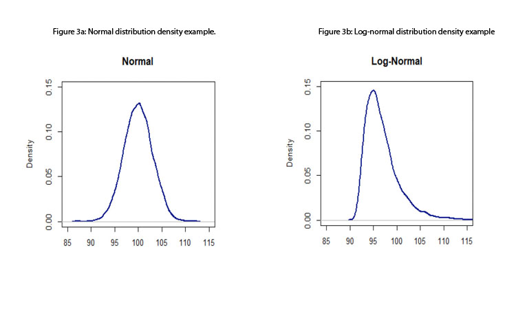
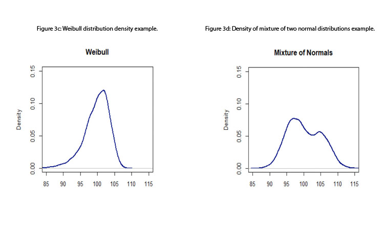
- Standard process capability or performance indices assume that the data come from a normal distribution; therefore, measurements are assumed to be independent of one another (otherwise, a time-series approach should be considered). Although this assumption is, in many instances, a reasonable one, the standard indices are not robust to departures from normality. 15 Figures 3a to 3d depict some distributions from quality attributes that may be observed in manufacturing process: skewed distributions (e.g., log-normal and Weibull distributions), multimodal distributions (e.g., mixture of two normal distributions), and unimodal with central tendency (e.g., normal distribution).
- Although nonparametric approaches for estimating capability indices exist, these have some limitations: 15
- The application of robust capability indices is essentially suitable for two-sided specification cases.
- Capability indices based on the percentiles of the fitted distribution rely on the appropriate identification and fitting of the distribution.
- Data-normalizing transformations are not always feasible and, in some instances, may not have a natural interpretation for practitioners.
- Capability indices based on resampling methods (such as bootstrap) have been shown to yield relatively poor results when distributions are highly skewed.
- Compendial test requirements are more complicated than the single-range specification used in process capability or performance indices. Compendial tests (e.g., the USP<905> test for uniformity of dosage, the USP<711> test for dissolution, and the USP<701> test for disintegration) can require multiple-stage testing and may include simultaneous constraints.
Given the preceding limitations, capability comparisons should be focused on assessing the probability of passing the test using either parametric or nonparametric assumptions. The use of nonparametric estimation techniques is suitable for CM because of the large density of data collected over time.
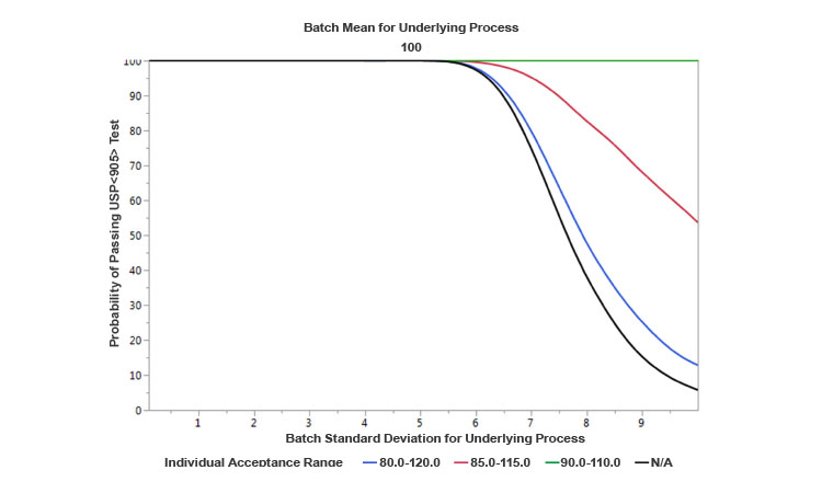
As a parametric example, Figure 4 provides a comparison of operating characteristics (OC) curves developed for the USP<905> test under the following assumptions: (a) One curve is based on normally distributed results with a fixed mean of 100, and variable standard deviations ranging from 0 to 10; (b) the other three curves reflect the existence of blending controls that divert material from the process to satisfy various target allowable ranges for individual uniformity of dosage units. The OC curves show that the narrower the window of allowable individual range due to more stringent controls is, the higher the probability of passing the USP<905> test is for the same expected level of underlying process variability prior to diversion. Therefore, conceptually, the appropriate level controls at the blending would tend to increase the capability of the process. Because these levels of controls can be implemented within a CM process and there are no hold times, product quality (and hence capability) can be improved relative to a traditional batch process. However, in some continuous processes with high natural variability, there could a trade-off: the increase in the capability could come at the cost of a reduction in yield (due to an increased waste of diverted material).
CONCLUSION
In a CM process, data from partial blends can be analyzed and suboptimal blends or tablets can be removed using the appropriate controls to avoid manufacturing issues downstream or out-of-specification final products. If these controls are implemented, a CM process could remove potentially unacceptable material, and the distribution of the critical quality attributes could result in improved process capability as compared to that of a batch process.
Data sources for CM controls include feeder controls and related models, chemical tests from physical samples, model-based predictions based on NIR spectroscopy or other similar technology, and indirect measures of the quality of the material obtained through physical sensors. Well-designed control systems will incorporate combinations of sensors and inline measures that span the process and either prevent quality aberrations or detect their existence. In some cases, physical sampling will be deemed necessary (and complementary) to verify that the process has not experienced any special-cause events. To determine the sampling frequency, one must consider the source of the measurements (e.g., physical samples vs. samples obtained using PAT tools), the development stage, and the measurement purpose (making local process-stage vs. batch-level quality statements).