Determining Number of Process Performance Qualification Batches Using Statistical Tools

This is the second discussion paper written by the ISPE Process Validation (PV) Team on the topic of determining and justifying the number of initial process qualification batches (e.g., FDA Stage 2, EudraLex Annex 15 process validation, EMA Guideline on process validation, etc.) needed to demonstrate a high degree of assurance in the product manufacturing process and control strategy, and thereby support commercialization of the product.
1 Introduction
This is the second discussion paper written by the ISPE Process Validation (PV) Team on the topic of determining and justifying the number of initial process qualification batches (e.g., FDA Stage 2 10, EudraLex Annex 15 process validation 13, EMA Guideline on process validation 14, 15 , etc.) needed to demonstrate a high degree of assurance in the product manufacturing process and control strategy, and thereby support commercialization of the product. Most regulatory authorities agree on implementation of the lifecycle approach to PV. The science- and risk-based approach to determining the number of batches for the PV exercise is preferable, as opposed to defaulting to three batches. Differences of opinion and questions remain about the best way to translate the risk-assessment results into the actual number of batches, including acceptable statistical methodology options and the required level of statistical confidence, if applicable.
The Team’s original discussion paper, “Topic 1 – Stage 2 Process Validation: Determining and Justifying the Number of Process Performance Qualification Batches (Version 2),” by Bryder, et al., was issued in August 2012 and updated in 2014 3. It featured three approaches to assigning an appropriate number of PV batches to risk-assessment results in an attempt to address the expectation outlined in the FDA PV Guidance of 2011 10, which stated that a high degree of assurance in the process must be obtained prior to release of commercial batches. This process assurance evaluation must also consider the result of process development (e.g., FDA Stage 1 10, EudraLex Annex 15 planning for qualification and validation 13) together with the results of the process-validation exercise (e.g., FDA Stage 2 10, EudraLex Annex 15 process validation 13). The three approaches presented in the first paper were useful in provoking thought and moving pharmaceutical industry understanding forward through various discussions, including discussions at scientific forums. As a result, several additional approaches have been developed, four of which are discussed in this paper.
2 Scope
The scope of this paper is limited to determining the number of initial PV, or Process Performance Qualification (PPQ) batches, using statistical tools identified in this paper. This paper supplements the “Topic 1 – Stage 2 Process Validation” Discussion Paper 3 which covers additional approaches in determination of number of PPQ batches.
This paper presents various statistical tools that can be used in determination of the number of PPQ batches. This paper will not attempt to explain basic statistics, but will present statistical tools with case studies or examples to demonstrate the use of the tool to arrive at the number of PV batches. Each statistical tool presented in this paper is intertwined with risk-based approaches, making it a hybrid approach. This paper assumes that a quality risk-management program is established, as described in ICH Q9, Quality Risk Management 6. Alternatively, the risk-assessment methodology presented in the “Topic 1 – Stage 2 Process Validation” Discussion Paper may be used 3.
Strategies presented in this paper may be modified as needed by manufacturers to suit their established systems, processes, procedures, and/or policies. Suggestions and recommendations presented in this paper are intended to furnish a wide range of tools in determining the number of PV batches. They are not intended to represent an industry consensus, nor is it the paper’s intention to present one as more preferable than the others, as each approach may have its own limitations.
The statistical approaches, in combination with the risk ratings presented in this paper, can be applied to both Active Pharmaceutical Ingredients (APIs) and drug products. However, the risk assessment should consider the differences in the subject (i.e., API versus drug product).
3 Background
The “Topic 1 – Stage 2 Process Validation” Discussion Paper 3 explains FDA’s revised guidance on process validation and provides a risk-based framework for determining the number of batches for process validation. It discusses three risk-based approaches and outlines the pros and cons of each. Summaries of the three approaches are presented below:
Approach #1: Based on Rationales and Experience
This approach seems quite reasonable, but does not use statistics in the determination of the number of batches (see Table 1). It suggests using rationales based on historical information and process knowledge.
Approach #2: Target Process Confidence and Target Process Capability
This approach uses statistics, but it is immediately applicable only to normally distributed data and those processes that are in a state of statistical control. Although transformations from non-normal to normal distribution are sometimes possible, identifying a suitable transformation method can be a matter of trial and error. In addition, the user needs to draw conclusions consciously so as to apply them to the original process that generated non-normal data. This approach recommends implementing improvements to the process at the end of the PPQ batches if an expected process capability index (Cpk) range is not met.
Approach #3: Expected Coverage
This is a nonparametric approach based on order statistics—the minimum and maximum observed results are referred to as x(1) and x(n), respectively—and the properties of intervals based on these order statistics. In particular, the expected probability of a future observation being within the range defined by [x(1), x(n)] is (n – 1)/(n + 1). Users of this approach should select an appropriate level of coverage that is most suitable to their processes.
It is apparent that there is no single approach that fits all scenarios or processes, and that additional approaches may be useful.
4 Statistical Approaches for Determination of the Number of Batches
4.1 Tolerance Intervals
FDA guidance states that “The number of samples should be adequate to provide sufficient statistical confidence of quality both within a batch and between batches.” 10 This statement prompts two questions:
- What is sufficient statistical confidence?
- How will the between-batch quality be measured?a
Both questions can be addressed by using tolerance intervals as PPQ protocol acceptance criteria for critical quality attributes (CQAs). Acceptance criteria in the PPQ protocol could be that the Tolerance Interval must be within the routine release criteria for the CQA (this may be the specification or a tighter internal requirement).
Tolerance intervals are intervals that cover a fixed proportion of the population (p) with a stated confidence (γ). A γ/p Tolerance Interval provides limits within which at least a specified proportion (p, also known as coverage) of future individual observations from a population is predicted to fall with a specified confidence level (γ). For example, a 95%/99% Tolerance Interval of 98.5 to 101.7 means that there is at least 95% confidence that at least 99% of future results will be between 98.5 and 101.7. For more information on tolerance intervals, refer to the NIST/SEMATECH e-Handbook of Statistical Methods 9.
All tolerance intervals discussed in this approach assume continuous normally distributed data, two- sided specifications, and k values approximated using the Howe method5. Additionally, it is assumed that the process is in a state of statistical control.
The confidence and coverage levels chosen should be based on a risk assessment, as in the “Topic 1 – Stage 2 Process Validation” Discussion Paper 3, where lower confidence and coverage levels are applied to a lower risk situation and higher confidence and coverage levels are applied to a higher risk situation. While all confidence and coverage selections are arbitrary, some minimum acceptable level should be stated. A level of 50% for either would be low. A floor of 80% is suggested, but this may be too low for certain companies or applications. Table 1 provides an example of how these levels might be assigned:
| Residual Risk Level | Confidence | Coverage |
|---|---|---|
| Severe (5) | N/A | N/A |
| High (4) | 95% | 99% |
| Moderate (3) | 95% | 95% |
| Low (2) | 90% | 90% |
| Minimal (1) | 85% | 85% |
Many other level assignments are possible. The key feature of any assignment is that the levels be non- decreasing with risk. It is also suggested that the confidence and coverage levels be fixed well in advance of PPQ activities. In this way, the focus can be uniquely on the risk assessment process.
To determine the number of batches (N) needed for PPQ, one additional value should be set. Looking at the general equation of a tolerance interval:
Y ± k * S where k = f ( y, p, N)
Where:
N = minimum number of PPQ batches: the total number of unique batch results included in the PPQ final report Tolerance Interval calculations. These results are not limited to batches run as part of PPQ, but can include previously identified stage 1 batches from comparable processes.
p = percent of the population to be contained in the Tolerance Interval.
γ = the statistical confidence that the Tolerance Interval contains p percent of the population.
f = a function where the inputs (γ, p, N) determine the output, k. This function is complicated and cannot be written in closed form.
k = output of f(γ, p, N). It is a constant, which when multiplied by S, determines the γ/p Tolerance Interval width.
S = standard deviation of the N results.
Y = the mean of the N results.
k is uniquely determined when three values (γ, p, N) are known. Similarly, when γ, p, and k are known, N is uniquely determined. It is this fact that will be used to determine the number of batches for PPQ in this approach. This fact can be summarized as:
k = f (y, p, N) ⇒N = f ( y, p, k)
Example: If γ = 95%, p = 95%, and k = 3.5, then N = f(95%, 95%, 3.5) = 10.
Interpretation: a 95%/95% Tolerance Interval needs a sample size (number of batches in this case) of at least 10 to have a k value no bigger than 3.5.
While choices for k are not extremely intuitive, reasonable values can be narrowed down based on common relationships. If k = 3.0, then the Tolerance Interval is the width of control chart limits (± 3 σ). If k were smaller than 3.0, then the Tolerance Interval would not “cover” the expected common cause variability. Therefore, k should be at least 3.0. At the other end, large values of k can be related to process capability measures. A k of 4.0 corresponds to a process performance index (Ppk) of 1.3, and a k= 6.0 to a Ppk = 2.0. While a Ppk = 2.0 (Six Sigma process) is a laudable goal, the final commercial specifications will likely be closer to 4 σ. Additionally, the smaller k is restricted to, the more conservative the final sample size for validation will be. While there is no absolute answer, it seems reasonable that k should be restricted to between 3.0 and 4.0. In this document, k = 3.5 will be utilized.
| Residual Risk Level | Minimum Number of PPQ Batches | Readily Pass Tolerance Interval | Marginally Pass Tolerance Interval |
|---|---|---|---|
| Severe (5) | Not ready for PPQ | N/A | N/A |
| High (4) | 24 | 95%/99% | 80%/80% |
| Moderate (3) | 10 | 95%/95% | 80%/80% |
| Low (2) | 5 | 90%/90% | 80%/80% |
| Minimal (1) | 4 | 85%/85% | 80%/80% |
“Minimum number of PPQ batches” refers to the total number of unique batch results included in the PPQ final report Tolerance Interval calculations. These results are not limited to batches run as part of PPQ, but can include previously identified stage 1 batches from comparable processes.b, 10
Example: A new monoclonal antibody (drug substance) is being validated for the first time. The associated company has chosen (in advance) to use the confidence and coverage levels from this paper (along with a k = 3.5). A team of scientists go through a risk assessment. The residual risk level is determined to be moderate. Using this, the minimum number of batches for PPQ is determined to be10. However, this can include previously identified stage 1 batches from comparable processes. It is determined that there are five such batches (three registration stability batches and two clinical trial batches). Therefore, at least five additional batches will need to be manufactured during PPQ. Criteria in the PPQ protocol for each quantitative CQA will be: 95%/95% Tolerance Interval on release results (all PPQ batches and five previously identified stage 1 batches) must fall within the acceptance criteria for the CQA.
If the 95%/95% Tolerance Interval is within the acceptance criteria for the CQA (i.e., readily pass criteria), then there is high confidence that the process can reproducibly comply with the CQA. Sampling and testing may be adjusted to a routine level in stage 3.
If the 80%/80% Tolerance Interval is within the acceptance criteria for the CQA (i.e., marginally pass criteria), then adequate confidence of quality in the CQA has been demonstrated between batches. Heightened monitoring and/or testing of the CQA is needed until a “readily pass” level of quality can be demonstrated for the CQA.
If the release results do not meet the “marginally pass” criteria, then the PPQ acceptance criteria has not been met and appropriate actions need to be taken before moving to stage 3.
4.2 Probability of Batch Success Approach
There are typically quite a few CQAs for each batch of drug substance or drug product, with specification limit(s) for each CQA. Examples of CQAs for drug substances include, but are not limited to, color, assay, related substances (impurities), moisture, residual solvents (such as ethanol or propanol), heavy metals, and particle size distribution. Examples of CQAs for drug products include but are not limited to appearance, assay, content uniformity, drug-related impurities, and tablet hardness and dissolution.
In this section we discuss using the probability that a batch will meet all of its specifications to determine the number of PPQ batches. This approach offers an intuitive and relatively simple methodology for determining the number of PPQ batches. In particular, it imposes no new process performance criteria (such as minimum values for process capability indexes) and naturally incorporates any number of specifications. It should be noted that this approach is particularly useful for high-volume processes with a large number of CQAs, all of which are likely to meet specification. The categorization of batches into successes and failures results in a loss of information that can increase sample size, and sample size may be further increased by batch failures.
Let 𝑝𝑖 represent the probability of meeting the ith specification, for i = 1, 2, … r specifications, and let 𝑝 represent the overall probability of a batch meeting all of its specifications. The value of p is a complex function of 𝑝1, 𝑝2, …, 𝑝𝑟, where each 𝑝𝑖 can involve both the true status of a CQA and measurement error. It may be tempting to think that 𝑝 = 𝑝1𝑝2 ⋯ 𝑝𝑟, but this expression ignores dependencies among the CQAs. For example, tablet hardness may be highly correlated with dissolution, and impurities may be correlated with one another. Fortunately, the approach used in this section does not need the individual values 𝑝1, 𝑝2, ⋯ , 𝑝𝑟. Instead, the binomial distribution is used to determine the probability of observing k successful batches in n independent trials:
𝑃(𝑘)= (n/k) 𝑝𝑘(1 − 𝑝)𝑛−𝑘
where k is the number of successful batches (i.e., the number of batches meeting all specifications), n is the number of batches produced, and 𝑝 is the overall probability of a successful batch.
Suppose we have observed k successful batches in n independent trials and wish to make a statement about the overall probability of success, 𝑝. Statistical inference for 𝑝 is a well-studied problem. A common estimator of 𝑝 is the maximum likelihood estimator 𝑝̂ = 𝑘⁄𝑛, and there are numerous methods for constructing confidence intervals for 𝑝 2. Some commonly used confidence intervals for 𝑝 are the Agresti–Coull interval 1, the Clopper–Pearson interval 4, the Jeffreys interval2, the Wilson score interval11, and the Wald interval.
The Wald interval is based on a normal approximation; it is easy to compute, but has poor coverage properties 2. The other four intervals have reasonably good coverage properties, but the Clopper– Pearson interval is the only one that guarantees the stated level of confidence. This guarantee comes at a cost however; Brown et al. deem the Clopper–Pearson interval “wastefully conservative” 2. In the remainder of this section we use either the Wilson score interval or the Jeffreys interval.
Bayesian statistical methodology can also be used to make inferences about the probability of success, 𝑝. Bayesian methodology allows one to formally include prior information about 𝑝 in the analysis. A Bayesian approach that utilizes an informative prior distribution for 𝑝 is discussed by Yang 12. Here we focus on using a non-informative prior in conjunction with a risk analysis, but note that an informative prior may be very useful when making minor modifications to an existing process. The well-known conjugate prior distribution for 𝑝 is a beta distribution with parameters (α0, β0). The parameter α0 can be thought of as the prior number of successful batches, and the parameter β0 can be thought of as the prior number of failed batches. The prior mean of 𝑝 is simply α0⁄(α0 + β0). Two popular non- informative priors are the Jeffreys prior (α0 = β0 = ½) and a uniform prior (α0 = β0 = 1). The ensuing posterior distribution for 𝑝 is also a beta distribution, with parameters (α1, β1) = (α0 + k, β0 + 𝑛 − 𝑘). It can be seen that the conjugate prior adds α0 successes and β0 failures to the observed results. Credibility intervals for 𝑝, a Bayesian version of confidence intervals, can be obtained using percentiles of the posterior distribution. The Jeffreys prior leads to the Jeffreys interval previously discussed in this section.
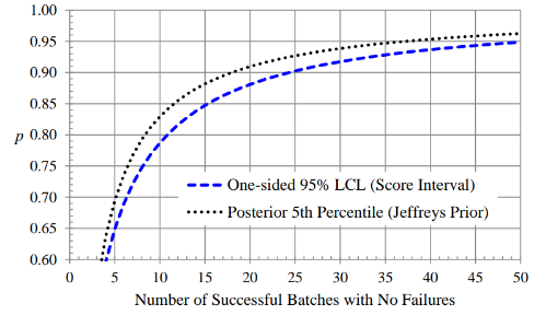
The number of PPQ batches can be based on statistical inference for 𝑝, the overall probability of a batch meeting all of its specifications. We focus on the situation in which we have observed n successful batches in n independent trials. Situations in which one or more batch failures have been observed will depend on the results of a root cause analysis and the perceived effectiveness of corrective and preventive actions. It is possible that some previous batch failures can be ignored if they are considered no longer probable. Figure 1 shows one-sided 80% lower confidence limits (LCLs) for 𝑝, based on the Wilson score and Jeffreys intervals, and Figure 2 shows one-sided 95% LCLs. Note that fairly large sample sizes are needed to obtain 95% confidence in a specific value of 𝑝, relative to 80% confidence. For example, using the Wilson score interval we are 80% confident that 𝑝 is at least 0.93 if we observe 10 successful batches in 10 independent trials, while we are 95% confident that 𝑝 is at least 0.92 if we observe 30 successful batches in 30 independent trials.
As an example of using the probability of batch success to determine the number of PPQ batches, suppose a project has completed 10 successful clinical batches with same process and formulation used in the regulatory filing, with no batch failures. Based on a risk assessment that results in a moderate level of residual risk, the project team has determined that they would like 90% confidence that the probability of batch success is 90% or greater. This requires a total of 15 batches with no batch failures, so the project team recommends five PPQ batches. If all five batches are successful, the process will be deemed validated and further information on process performance will be obtained in stage 3 (continued process verification). Sample sizes for additional levels of residual risk are illustrated in Table 3, which is provided for illustrative purposes only. Table 4 provides a Bayesian version based on the Jeffreys prior. These tables show that a large number of batches are needed to obtain high levels of confidence in 𝑝. Consequently, manufacturers should give considerable thought to the level of confidence that is needed for a specified residual risk, and develop their own versions of Table 3 and Table 4.
Figure 1: One-Sided 80% Lower Confidence Limits for 𝒑
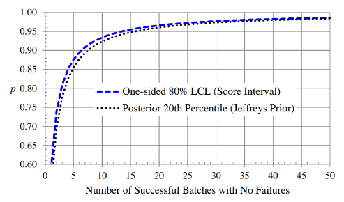
Figure 2: One-sided 95% Lower Confidence Limits for 𝒑
| Residual Risk Level | Total Number of Batches with No Failures | Confidence Level | One-sided LCL for 𝒑 |
|---|---|---|---|
| Severe | N/A | N/A | Not ready for PPQ |
| High | 24 | 95% | 89.9% |
| Moderate | 15 | 90% | 90.1% |
| Low | 10 | 85% | 90.3% |
| Minimal | 7 | 80% | 90.8% |
| Residual Risk Level | Total Number of Batches with No Failures | Confidence Level | One-sided LCL for 𝒑 |
|---|---|---|---|
| Severe | N/A | N/A | Not ready for PPQ |
| High | 18 | 95% | 90.0% |
| Moderate | 13 | 90% | 90.3% |
| Low | 10 | 85% | 90.4% |
| Minimal | 8 | 80% | 90.5% |
Note: If one or more of the CQAs poses a significant risk of not meeting specification, it might be more useful to examine those sub-processes in more detail and use an alternative approach to PPQ sample size, or perhaps to model the probability of meeting those specific specifications, as in LeBlond and Mockus 7.
4.3 Combinational Approach of Analysis of Variance with Risk Assessments
For this approach to determine the number of batches required, the observed variation from stage 1 batches is partitioned into the within-batch and between-batch components. Data from commercial scale engineering/demo batches would be the ideal data set to analyze. However, this may not be possible, and thus the user should use scientific and technical expertise when determining if smaller scale batch data can be used. The between-batch component is then used with a National Institute of Standards and Technology (NIST) based calculation to determine finally the number of batches required. Using just the observed variation could overly estimate the number of required batches, thus increasing costs and lengthening the time required to complete the validation study. FDA process validation guidance 10 states that between-batch and within-batch variability needs to be understood. This could be in terms of what can cause these variabilities and could include the ability to quantify them.
The main prerequisite needed is to understand what “shift” in the mean response of the parameter is considered to be of practical significance. The baseline for the shift consideration is the mean of the response of the attribute as seen in the demo or engineering runs. Because specification limits were used during the manufacturing of phase I and phase II batches, one suggestion would be to define this shift in mean as a percentage of the specification window, and leverage some form of risk analysis that looks at the criticality of the quality attribute in question, as well as the residual risks identified after a control strategy has been identified (via formal risk assessment) and implemented. Figure 3 and Figure 4 summarize this approach.
Figure 3: Risk Index Identified for Each Quality Attribute and Residual Risk Interaction
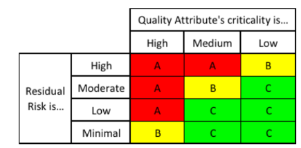
Using the risk index from Figure 3, the respective shift can be determined as seen in Figure 4:
Figure 4: Recommended Shifts to be of Practical Significance
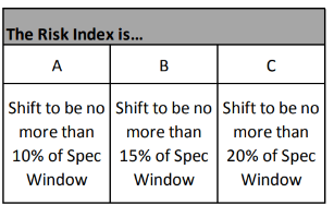
The values of 10%, 15%, and 20% are selected based on the risk of significantly changing the Cpk and hence the out of specification product being produced. Table 5 shows how out of specification (OOS), parts per million (PPM) failure, and Cpk change as the shifts get bigger. Table 5 was calculated using the Statistical software, JMP, which is a product of the SAS company using Avg. = 100; Std. Dev = 2, USL = 110, and LSL = 90.
| % of Spec Window | Actual Shift | Cpk | OOS | PPM Failure | Change in Cpk |
|---|---|---|---|---|---|
| 0.00% | 0 | 1.67 | 0.0000287% | 0 | 0.00% |
| 10.00% | 2 | 1.33 | 0.0031671% | 32 | -20.00% |
| 15.00% | 3 | 1.17 | 0.0232629% | 233 | -30.00% |
| 20.00% | 4 | 1.00 | 0.1349898% | 1,350 | -40.00% |
As the criticality of the attribute goes up, the acceptable mean shift to be seen, if it exists, gets smaller.
Given this understanding of a mean shift that is practically significant, the flow map in Figure 5 can be constructed to determine the minimum number of batches to be run for validation, as well as minimum samples to be taken per batch.
Figure 5: Flow Map to Determine Minimum Number of Batches
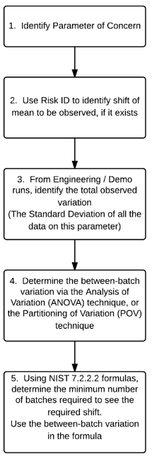
Once the mean shift to look for has been identified, one can use section 7.2.2.2 of the NIST/SEMATECH e-Handbook of Statistical Methods9 to calculate the minimum sample size required. The between- batch variation can be determined using the approach discussed by Little 8.
Example: Data for CQA1 for product “W” gave the graph, as seen in Figure 6, for five engineering batches. The specification for the CQA1 is 90 – 110.
These engineering batches were executed by including as much input (raw materials, operators, environmental conditions, non-key process parameters) variation as possible.
Figure 6: Plot of CQA1 from Five Batches of Product “W”
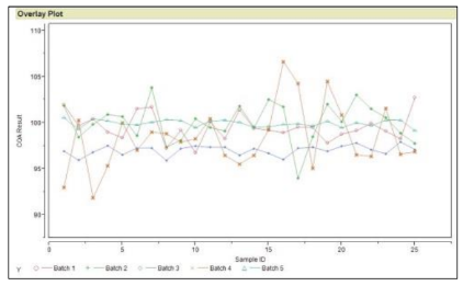
Figure 7: Analysis of Variance (ANOVA) and Process Output Variable (POV) Breakdown
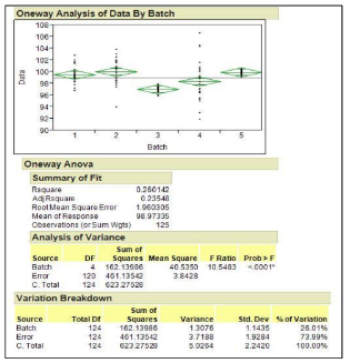
From Figure 7, using the POV analysis (sum squares/total Df = variance) one can tell that 26% of the overall variation comes from between-batch variation, and the rest (74%) comes within-batch variation. In addition, one can determine that the total observed standard deviation is 2.242 and the total variance is 5.0264.
Now, to determine the shift in the mean response of the parameter, given that this is a CQA with a specification of 90 to 110, the desired shift in mean is determined to be no more than 10% of the specification window or [0.1 × (110 – 90)] = < 2.0.
Table 6 shows the calculations based on the NIST/SEMATECH e-Handbook of Statistical Methods 9.
| USL | 110 |
| LSL | 90 |
| Tol | 20 |
| Mean shift that is of Practical Significance | 2 |
| Total Variation | 5.026564 |
| % var (between batch) | 26.00% |
| Between Batch Var | 1.30690664 |
| Between Batch S.D. | 1.143200175 |
| alpha | 0.05 |
| Beta | 0.1 |
| 1-beta = | 0.9 |
| z(1-beta) = | 1.28 |
| 1-alpha/2 = | 0.975 |
| z (1-alpha/2) = | 1.96 |
| N1 = | 4 |
| N | 4 | 8 | 5 | 7 | 5 | 7 | 5 | 7 | 5 | 7 |
| t(1-alpha/2) | 3.182 | 2.365 | 2.776 | 2.447 | 2.776 | 2.447 | 2.776 | 2.447 | 2.776 | 2.447 |
| t(1-beta) | 1.638 | 1.415 | 1.533 | 1.440 | 1.533 | 1.440 | 1.533 | 1.440 | 1.533 | 1.440 |
| New N | 8 | 5 | 7 | 5 | 7 | 5 | 7 | 5 | 7 | 5 |
| Number of batches required 6 |
Using the NIST approach and the POV variation analysis method suggested by Little8, one needs a minimum of six batches to clearly see a shift in mean of 10% of the specification window, if this shift exists.
A similar approach was conducted for the remaining two CQAs and the 2 parameters of medium criticality. Table 7 summarizes the results of each.
| CQA | Min. Number of Batches Required |
|---|---|
| CQA1 | 6 |
| CQA2 | 5 |
| CQA3 | 4 |
| Med4 | 3 |
| Med5 | 4 |
For this particular product, running a minimum of six batches for validation will allow seeing the required mean shifts, should they exist. The validation protocol can contain an acceptance criteria to specify “The mean of <<Quality Attribute 'A'>> should be between X ± S” where X is the mean value of the quality attribute as derived from the demo/engineering studies, and S is the shift in mean that is of practical significance. If the value of the mean of the combined batches is outside of this range, then an investigation should be conducted to understand why this is so and appropriate actions should be taken. It goes without saying that this should be one of several acceptance criteria to judge the success of the validation.
One of the limitations of this approach is that it is not possible to make confidence statements such as “X % confidences that Y% will be within specification”. The intent of the outlined approach was never to show that the lots would be within specification; that should have been demonstrated as part of stage 1 development and engineering studies. Instead, the intent of this approach is to show a consistent performance of the process being validated and that there is no difference between the commercial scale process at stage 1 and stage 2. Another limitation of this approach is that the stage 1 batches are assumed to be at commercial scale, which may not be common for small-molecule manufacturing. One unintended consequence of this approach is that the shift in mean to detect could be widened. This would lead to fewer batches being needed for stage 2 purposes.
4.4 Variability Based Approach
One criterion for a successful validation is that the process exhibits low variability. In this approach, a predetermined estimate of variability is used as the basis for selecting the number of batches for validation.
This approach is applicable when validating a process following a significant change to the current process or when a process is being transferred from one site to another. In such cases, there is a well- established estimate of process variability based on the historical process data. The goal of the validation is to ensure that the process being validated continues to show variability similar to, or no worse than, the current process. Although it is important for the process average to remain on target as well, there may be differences between the current and new process averages due to factors such as equipment, setup, and raw materials being used. This approach assumes that adjustments to achieve the target process average can be made more easily once the process variability is deemed acceptable.
If the current process has been stable prior to the PPQ, the historical estimate of variability from that process can then be thought of as a “known” parameter or a population value. If the data from validation batches can be shown to have the same variability as the current process, the estimate of variability from the current process can be used to determine the capability of the process being validated.
A power curve is used to select a sample size to test the hypothesis that the ratio of the sample standard deviation to the population value is no more than a specified value R. The hypothesis to be tested is
Ho: (SDV/σp) ≤ R
H1: (SDV/σp) > R
Where:
R = ratio of validation standard deviation to historical population standard deviation
H = null or alternative hypothesis
SDV = the standard deviation associated with the validation batches
σp = the known standard deviation from the historical batches of the current process.
The confidence level (1 – α) and power (1 – β) should be specified, where α is the probability of rejecting the null hypothesis when it is true and β is the probability of accepting the null hypothesis when it is false.
The choice of R depends on the process knowledge available, including the impact of the process change to the process being validated. A value of 2 can be used as a good rule of thumb to indicate similarity of variability, especially when the risk to the process is low. A lower value of R may be preferred when risk is high.
The choice of α and β will also depend on the identified residual risk. For example, for quality attributes that are associated with moderate risk, smaller α and β values may be chosen (e.g., 0.05 and 0.2 respectively), whereas for quality attributes that are associated with lower risk, higher α and β values may be chosen (e.g., 0.05 and 0.3 respectively). Higher values of β mean that there is greater probability that we would find the validation variability acceptable when it is actually unacceptably high. If the validation is being performed for a technology transfer or after changes to the current process, the residual risk is generally determined to be small due to the abundance of information available from the current process. The number of batches for a given residual risk is summarized in Table 8; the risk levels listed are consistent with those defined in the “Topic 1 – Stage 2 Process Validation” Discussion Paper 3, as well as the topics discussed in this paper. Other choices of α and β are possible, and these should be determined by each organization during their risk assessment process.
| Residual Risk Level | Ratio | Target Confidence Level | Target Power | Number of Batches |
|---|---|---|---|---|
| Severe | N/A | N/A | N/A | N/A |
| High | 2 | 95% | 90% | 11 |
| Moderate | 2 | 95% | 80% | 8 |
| Low | 2 | 95% | 70% | 6 |
| Minimal | 2 | 80% | 70% | 4 |
Note: There is a certain level of arbitrariness in selecting a particular confidence level or power for a given risk level. It is up to the organization to decide whether the chosen confidence level and/or power are consistent with their understanding of the risk level identified and impact to the process and/or product.
For example, if eight validation batches are run for a moderate risk level, there is an 80% chance of detecting a ratio exceeding 2.
If the product being validated has multiple variants, the total number of batches may be made up across the different variants, as appropriate. Based on the risk assessment, certain variants may be replicated more than others. The total number of batches may also include process development batches or any other batches made by the same manufacturing process as that used for stage 2. Statistical analysis should be performed on the data collected for the CQAs. A test of hypothesis should be performed on the sample SDV to determine whether its ratio to the historical standard deviation (σp) does not exceed a specified value. If multiple variants have been used, then it may be possible to combine data for some CQAs across some or all variants, as these CQA values do not vary across the variants. This helps ensure appropriate power for the analysis.
If the null hypothesis is not rejected and the ratio does not exceed the specified value, the validation batches may be considered to be no different from the current process with respect to the standard deviation, and the historical estimate of the process standard deviation can be used for any further evaluation of the process, fe.g., in calculating process capability. Since a known estimate of variability is being used, there is less uncertainty in the estimate of process capability.
If the null hypothesis is rejected and ratio is greater than the specified value, the standard deviation of the validation batches is unacceptably higher than that of the current process. In this case, additional work may be needed to better understand and mitigate the sources of variability before validation can be considered complete.
Additional analyses should be performed to assess the capability of the process using the historical estimate of the standard deviation and the sample mean from the validation batches. These should be determined when planning the process validation and will depend on the risk assessment performed. Various analyses and/or criteria for passing validation are possible; some of which are mentioned below:
- All validation batches are within specification
- Calculate Cpk and compare it to historical Cpk
- Calculate Cpk and compare against a stated acceptance criteria
If Cpk is being calculated, then the target Cpk values should be determined by the organization prior to validation, based on the product being validated. Acceptance criteria based on Cpk were previously proposed in the “Topic 1 – Stage 2 Process Validation” Discussion Paper 3 and may be used to judge the validation. These criteria use the confidence interval for the Cpk to determine the acceptability of the batch; this is necessary since very few batches are available for this calculation, leading to greater uncertainty in its estimate. An example is provided in Table 9 using the number of batches proposed in Table 8.
| Residual Risk Level | Number of Batches | Target Lower Confidence Bound for Cpk | Acceptance Criteria | ||
|---|---|---|---|---|---|
| High | 11 | 95% | If Cpk ≥ 1.6, readily pass validation | If 1.0 ≤ Cpk < 1.6, marginally pass/more work needed | If Cpk < 1.0, fail validation |
| Moderate | 8 | 90% | |||
| Low | 6 | 85% | |||
| Minimal | 4 | 80% | |||
If the observed Cpk ≥ 1.6, the true Cpk value is at least 1.0 in each case above. Thus, there is high confidence that the sample mean is also close to the target value; in this case, we can consider the validation to have passed easily, and enhanced monitoring may not be necessary. However, since the validation batches may not represent all sources of process variability, the process variability should continue to be monitored to ensure that it continues to meet the target set for validation. If the 1.0 ≤ Cpk< 1.6, there is less confidence that the process mean is at or close to target and further work is needed to a) better understand and improve the mean, and b) to reduce the variability further, as needed. The process should be evaluated further to identify and/or adjust process parameters that impact the mean. Depending on the residual risk associated with the process, this may be done before validation can be considered complete or during the enhanced monitoring stage. Finally, if Cpk < 1.0, the process is at high risk of producing OOS batches during manufacture and cannot be validated.
The approach provided assumes that the process is stable and the data are normally distributed. These assumptions should continue to be verified as more data become available during enhanced or routine monitoring.
Example: Validation was to be performed on an existing manufacturing process following a significant change to the process. The existing process had been used for a long time and there was a wealth of information and data for this process. The product was made in two batch sizes, had three strengths, and was sold in two market segments with slightly different manufacturing requirements.
During the risk assessment process, which included analyses of nearly 2 years of historical data, the following was concluded:
- Ten of the 12 combinations of product/process needed to be evaluated during validation; therefore, a minimum of 10 batches would need to be run. The remaining two combinations were not going to be manufactured.
- Some CQAs could be combined across all combinations; these did not vary across markets or strengths, and were made to the same specification. Others could only be combined for markets or only for product strength.
- Some CQAs show more variability for some combinations than others.
- Not all CQAs are equally critical from a validation impact perspective; some were impacted by the change to the process while others were not.
The risk analysis resulted in the selection of a minimum power of 80% to test the ratio of the standard deviations for various CQAs. Thus, the smallest number of batches needed for any CQA was 8. In order to achieve this power, the following replicates were run (see Table 10):
| Product Strength | Market 1 | Market 2 | ||
| Batch Size 1 | Batch Size 2 | Batch Size 1 | Batch Size 2 | |
| 1 | x | 2 | x | 2 |
| 2 | 2 | 2 | 1 | 1 |
| 3 | 2 | 2 | 2 | 2 |
Based on the risk assessment performed, for one CQA (assay), variability for product strength “3” was evaluated on its own using eight batches by combining markets and batch size, while variability for product strengths “1” and “2” was evaluated using 10 batches by combining strengths, markets, and batch size. For other CQAs, all 18 batches were used in the evaluation.
5 Conclusion and Further Discussion
The approaches presented in this discussion paper use a combination of statistics and risk assessments, making them hybrid approaches for determining the number of PPQ batches. Four possible approaches are presented with examples and/or case studies.
A Tolerance Interval approach is presented that recommends using tolerance intervals as the PPQ protocol acceptance criteria. Using risk assessments, the confidence and coverage levels may be determined, lower confidence and coverage levels may be applied to a lower risk situation, and vice versa.
The probability of batch success approach described in this paper provides a starting point that is particularly useful for a high-volume process with a large number of CQAs, none of which pose a significant risk of not meeting specification. This approach incorporates any number of specifications without imposing any additional process performance criteria, such as minimum values for process capability indexes.
The combinational approach of analysis of variance approach with risk assessments presented in this paper is based on the shift in the mean response of the key parameter or CQAs. The number of PPQ batches required is estimated by determining the between-batch variation using an ANOVA or POV technique and utilizing NIST 7.2.2.2 formulas 9 for the required shift in mean of a key parameter or CQA.
The variability-based approach presented in this paper is based on the historical variability and the selection of the target ratio, confidence level, and power appropriate with residual risk. This approach is applicable to processes that undergo a significant change or have been transferred from one site to another.
Other approaches may be used, and industry is encouraged to collaborate further with ISPE to support progress in the PV lifecycle approach.
Limitation of Liability
This discussion paper is presented as supplement to the original discussion paper that was issued in August 2012, “Topic 1 – Stage 2 Process Validation: Determining and Justifying the Number of Process performance Qualification Batches (Version 2)” proposing ideas for answering the question “How many process performance qualification batches (PV stage 2) are needed to demonstrate a high degree of assurance in the manufacturing process and that the control strategy is sufficiently robust to support commercial release of the product”. The purpose of this paper is to present four (4) statistical tools that may be applied to determine the number of PPQ batches. This paper discusses the statistical approaches, their limitations, assumptions, and also presents simulated examples. Considerable input has already been received, considered, and/or incorporated. The author team is interested in hearing about other approaches that could be used, and lessons from use of the proposed approaches described in the discussion paper and additional examples. The paper may be modified or expanded sometime in the future to reflect additional input.
Please direct all feedback to pvpapers@ispe.org.
Acknowledgements
Christopher Breen (Eli Lilly),
Dilip Ayyala Somayajula (Grand River Aseptic Manufacturing)
Maneesha Altekar (AstraZeneca)
Pritesh Patel (Pritesh Patel Consulting, LLC)
Richard A. Lewis (GlaxoSmithKline)