Cleanroom Recovery Study: Using Computational Fluid Dynamics Methodology
Computational fluid dynamics (CFD) can reduce or eliminate the uncertainty associated with a cleanroom facility as the planned design can be simulated to predict performance to a high degree of accuracy. This article discusses the use of CFD for the purpose of predicting and optimizing the performance of a cleanroom facility in terms of steady-state airborne particulate levels and for estimating the recovery time to a particulate challenge per ISO 14644-3.
An equation is derived to predict the recovery time for a cleanroom that is challenged with 0.5-micron particulates. The results from CFD are compared to the derived equation and to experimental data for a cleanroom waste airlock. A further CFD model of an entire cleanroom facility is made, and the recovery results are compared with the mathematically derived model.
The methodology presented here allows for particulate levels and recovery times to be estimated during the design phase of a cleanroom facility. This study illustrates that CFD is a valuable tool in reducing the uncertainty associated with a cleanroom design. Once created, the CFD model can be used for parametric studies to optimize a design. Design parameters such as air change rates, exhaust rates, supply and exhaust register locations, and supply register types (e.g., laminar, radial) can easily be studied to gauge the impact to particulate levels. These simulations were performed with ANSYS CFX software, version 2021R1.
Computational Fluid Dynamics Methodology
To gain confidence in the CFD methodology, a cleanroom waste airlock was first modeled for recovery time and compared to a mathematical model and experimental data. Even though a waste airlock is used in this study, the methodology formulated here applies equally to higher grade room classifications, such as an aseptic filling area. This work includes a mesh independence study on the CFD model, which compares particle recovery times for increasing levels of mesh refinement.
After a satisfactory agreement was made between the CFD model and experimental data for the airlock, a more complex facility was modeled and optimized to minimize the overall steady-state particulate level.
This article first analyzes a cleanroom waste airlock and then an entire facility composed of cleanrooms. Design input parameters for the waste air-lock came from the as-built/as-left condition (e.g., final air balance, field measurements) to align with the actual conditions. For a new construction, detailed or conceptual design parameters would be used to predict the cleanroom performance.
Mathematical Model
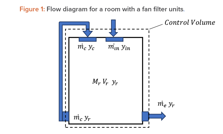
Figure 1 illustrates a typical cleanroom with a recirculation fluid stream that is part of a fan filter unit. The figure shows two filters, one part of the fan filter unit (associated with yc) and the other part of the outside air (associated with yin).
Assuming uniform particulate levels throughout the room, the concentration mass balance for the control volume in Figure 1 becomes:
\(\text{Equation 1:}\frac{dM_ry_r}{ dt}= \dot{m}_cy_c + \dot{m}_{in} y_{in} - \dot{m}_cy_r - \dot{m}_ey_r \)
Where: \(\dot{m}_i \) is the mass flow rate for stream i
- \(y_i \) is the particulate concentration for stream i
- \(M_r \) is the fluid mass in the room
Further, assuming that the flow is incompressible, in that there is a negligible impact of density as the variation in pressure is insignificant, and the room mass remains constant, Equation 1 becomes:
\(\text{Equation 2:} V_r\frac{dy_r}{ dt}= Q_cy_c + Q_{in}y_{in} - Q_cy_r - Q_ey_r \)
Where: \(Q_i \) is the flow rate for stream i and \(V_r \) is the room volume.
A mass balance reveals that \(Q_{in} \) = \(Q_e \).
In addition, if we let X = 1 – HEPA%, then yc = X yr and the equation becomes:
\(\text{Equation 3:} V_r\frac{dy_r}{ dt}= Q_cXy_r + Q_{in}y_{in} - Q_cy_r - Q_{in}y_r \)
Rearranging and integrating, the equation becomes:
\(\text{Equation 4:} \int\frac{dy_r}{ y_r(Q_cX-Q_c-Q_{in})+ Q_{in}y_{in}} = \int\frac{dt}{ V_r} \)
Integrating yields:
\(\text{Equation 5:} \frac{1}{(Q_cX-Q_c-Q_{in})}ln[y_r(Q_cX-Q_c-Q_{in}) + Q_{in}y_{in}] = \frac{t}{ V_r} + Const1 \)
Solving for time t, the above equation becomes:
\(\text{Equation 6:} t = \frac{V_r}{(Q_cX-Q_c-Q_{in})}ln[y_r(Q_cX-Q_c-Q_{in}) + Q_{in}y_{in}] = Const2 \)
At time t = 0, the room concentration \(y_r \) = \(y0 \) (initial concentration) and thus the Const2 is:
\(\text{Equation 7:} Const2 = - \frac{V_r}{(Q_cX-Q_c-Q_{in})}ln[y_0(Q_cX-Q_c-Q_{in}) + Q_{in}y_{in}] \)
Thus, the time equation becomes:
\(\text{Equation 8:} t (y_r) = \frac{V_r}{(Q_cX-Q_c-Q_{in})}ln [\frac {[y_r(Q_cX-Q_c-Q_{in}) + Q_{in}y_{in}}{y_0(Q_cX-Q_c-Q_{in}) + Q_{in}y_{in}} ] \)
The equation above provides the elapsed time in going from an initial room concentration \(y0 \) to a final room concentration \(y_r \). The equation can be used to estimate recovery times where \(y0 \) = 100 \(y_r \). Note this equation was formulated for a room with recirculation fan filter units but can easily be applied to a single-pass flow system with \(Q_c \) = 0.
Waste Airlock Modeling Using Closed-Form Solution
This waste airlock model consisted of a single-pass system with two doors, one HEPA inlet, and one exhaust. Since the airlock operated as a pressure sink, the model needed to account for the inlet flows across the doors, as this would affect the room particulate concentration. An easy way of accounting for these flows was to make \(Q_{in} \) and \(y_{in} \) a flow-weighted average of the infiltrated door flows and the HEPA inlet flow. As an example, if the infiltrated door flows are 50 cfm and 100 cfm at a concentration of 1,000 particles/m3 and 100,000 particles/m3, respectively, and the inlet HEPA air contains a flow of cfm at a concentration of 50 particles/m3, then \(Q_{in} \) would be set to 650 cfm with \(y_{in} \) set at 15,500 particles/m3.
To estimate the infiltrated door flows, design documentation can be used. Specifically, the differential pressure (dp) between rooms should be known from the pressurization plan, and design drawings can be used to estimate the flow area of the door clearance (gap between door edge and floor or door edge and wall).
In this study, to reduce the uncertainty of this methodology, field measurements were used for both the dp across the doors and the door clearance. The door infiltration flow rate is calculated based on the Darcy–Weisbach equation shown below, with the loss coefficient K simply modeled at 1.5, which is equal to an abrupt entrance + exit loss coefficient:
\(\text{Equation 9:} dp = \frac{1}{ 2} = \rho K (\frac{Q}{ A})^2 \)
Where: dp = differential pressure across the door:
- K = loss coefficient across door
- A = flow area of door clearance
- Q = door infiltration flow rate
- \(\rho \) = air density
Solving for the flow rate yields:
\(\text{Equation 10:} Q = A \sqrt{ \frac{2 dp}{\rho K}} \)
Using the above equation, the door infiltration flows were calculated.
Other field measured data that were used as inputs to Equation 8 are listed below:
- The HEPA inlet flow per air balance report
- Initial room concentration, \(y_0 \), per field tested recovery study
- Final room concentration, \(y_r \), per field tested recovery study
- Measured room volume
The waste airlock was designed as a single-pass system; therefore, the recirculation flow, \(Q_c \), in Equation 8 was set to zero. This equation estimated the waste airlock to take 7.24 minutes to go from an initial concentration of 100x to a final concentration of 1x.
Waste Airlock Modeling Using Computational Fluid Dynamics
As previously discussed, this room acts as a pressure sink, meaning that it operates at a lower pressure than the adjacent rooms. Thus, there is air infiltration into the room via the door clearances. The CFD modeled the doors in their closed position with air allowed through the bottom door clearance. The same flow rates that were used for the mathematical model were used for the CFD model. Two models were solved: first a flow-only model and then a particulate transient model. It is important to have the flow structure resolved before introducing the particulate challenge, otherwise the results may not be as accurate. The particulate transient started with flow results based on the steady-state flow-only solution with an initial particle concentration at 100x.
Assumptions
The following assumptions were made in our study:
- The air was assumed incompressible with properties at 25°C (77°F). The pressure changes are minor, so this assumption will not have a noticeable impact.
- Particle deposition does not typically occur for 0.5-micron-sized particles (medium-sized particles) as they typically flow with the air stream,2 thus particles are assumed to be fully suspended.
Selected Conditions
For this study, the following conditions were used:
- Isothermal conditions were used because there were no significant heat loads.
- To model turbulence, the two-equation RNG k- \(\epsilon \) model was used with medium turbulence intensity (5%), which is the recommended CFX option when no turbulence intensity information is available. As a check, the turbulence intensity formula, I = 0.16Re-1/8, for fully developed flow within a pipe was solved for the HEPA inlet flow and the door infiltration flows (with a hydraulic diameter = 4 × flow area ÷ wetted perimeter) and an intensity of approximately 5% was calculated.
- All physical walls contained a no-slip boundary condition, per boundary layer theory.
- The high-resolution scheme was used for turbulence and advection. This scheme uses second-order numerical modeling and is the recommended scheme to use for final results.
| Parameter of Interest |
Coarse Mesh | Medium Mesh | Fine Mesh |
|---|---|---|---|
| Number of Elements | 70,066 | 140,427 | 280,146 |
| Number of Nodes | 15,579 | 30,004 | 57,418 |
| y+ Area Average | 49 | 39 | 31 |
| Element Size (inch) | 4.7 | 3.0 | 2.2 |
| Recovery Time (min) | 9.30 | 9.47 | 9.45 |
Mesh Independence Solution
An unstructured mesh using mostly tetrahedral elements was applied with some prisms and pyramids as required. Two layers of mesh inflation using prisms were added off the floor to better capture the high-velocity gradients arising from the infiltrated door flows.
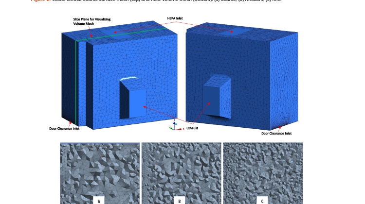
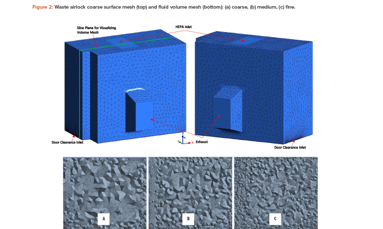
Three separate meshes were created to test mesh independence on recovery time. Successive mesh refinements doubled the total number of elements; the medium mesh had twice the number of elements as the coarse mesh, and the fine mesh had twice the number of elements as the medium mesh. Local mesh sizing was added to the door clearance. The local mesh-sizing parameters on the door clearance and the two-layer mesh inflation thickness did not change across the different meshes, only the global mesh size changed. Figure 2 illustrates surface mesh and volume mesh.
Table 1 shows the results of the mesh study for coarse, medium, and fine on the parameter of interest.
The results suggest that mesh independence was achieved with the coarse mesh, as the medium mesh results differ by less than 2% and the recovery time did not significantly change with a further doubling of the mesh density (fine mesh results). Thus, a global element size of 4.7 inches was sufficient to properly capture the flow physics along with the two-layer prisms off the floor and local mesh controls at the door clearance.
Mathematical Model, Computational Fluid Dynamics, and Experimental Data
The mathematical recovery time model and CFD agree within approximately 24% (7.24 vs. 9.47 minutes). The mathematical model was based on uniform distribution, and the CFD results were made based on a volume average concentration for an equal basis comparison. Though the CFD model did show that uniform particulate distribution did not exist, it was expected due to the existence of different particle concentrations for the inlet streams and the fact that mixing does not occur instantaneously.
The experimental data was taken at three different points within the waste room at approximately working level or about 3 feet from the floor. The experimental recovery times for these three points were 9 minutes, 10 minutes, and 9 minutes; averaging yields a recovery time of 9.33 minutes. The experimental results and CFD are in close agreement at less than 2% difference. This illustrates that, with the methodology provided in this CFD study, accurate predictions for particulate recovery times may be obtained using CFD.
Facility Computational Fluid Dynamics Model
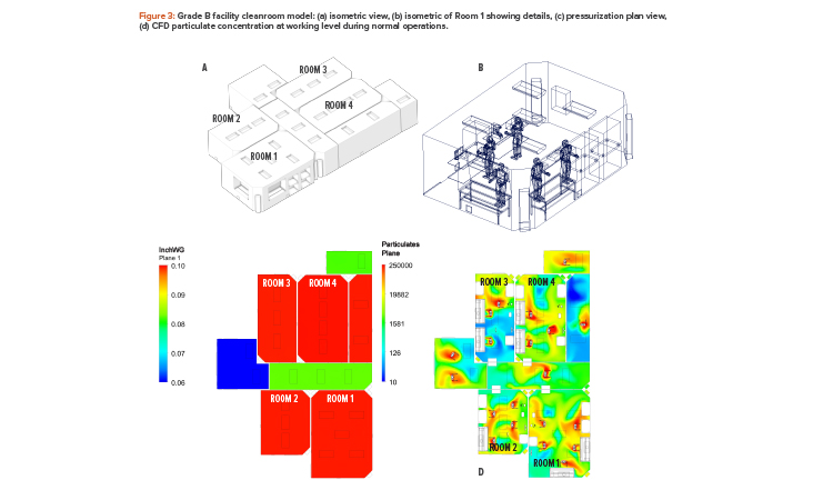
The CFD methodology discussed previously was implemented in a much larger cleanroom facility with four Grade B processing cleanrooms, a storage room, an entrance corridor, personal access, and material access, as shown in Figure 3. Radial HEPA supply registers were used in the model, and several rooms contained recirculating fan units.
| Room | CFD (min) | Experimental (min) | Difference (%) |
|---|---|---|---|
| Waste Airlock | 9.47a | 9.33 | 1.5 |
| Room | CFD (min) | Mathematical Model (min) | Difference (%) |
| Waste Airlock | 9.47a | 7.24 | 23.5 |
| Processing Room No. |
CFD (min) | Mathematical Model (min) |
Difference (%) |
| 1 | 5.32 | 6.19 | 16.4 |
| 2 | 5.15 | 6.02 | 16.9 |
| 3 | 5.60 | 5.84 | 4.3 |
| 4 | 5.27 | 6.02 | 14.2 |
The Grade B cleanrooms, shown in red in Figure 3, acted as bubbles, i.e., at higher pressure than adjacent rooms. The arrows shown in the pressurization plan view of Figure 3 illustrate the flow cascade and denote the door locations.
The recovery times were estimated using the mathematical model and CFD. This facility study included the following three elements:
- An operating study with personnel present to determine steady-state particulate levels; this included several different configurations for cleanroom optimization.
- A transient with no personnel to capture a steady-state flow condition, based on the final configuration from element A.
- A transient particle recovery study (no personnel present) with initial flow conditions from element B and a 1E8 particles/m3 starting concentration.
Element A of the study involved performing several simulations, each with a different configuration (such as different supply and exhaust locations), with the goal of reducing the steady-state particulate level; the final design is illustrated in Figure 3. For this study, personnel were modeled with an applied particulate generation source. A total of 20 personnel working in the facility was assumed, each generating 3,000 particles/second of 0.5-micron size, which was applied uniformly. This particle generation rate was considered conservative because people in Grade B cleanroom coveralls will generate no more than 1,000 particles/sec.3 To model the particle generation rate, a small velocity (such that it did not affect the room air change rate) was applied on personnel with a particle con-centration determined as below:
Particle Concentration = (3,000 particles/sec) ÷ (small velocity × surface area of person)
In addition to modeling personnel, the planned equipment (e.g., biological safety cabinets, tables, chairs) was also modeled. Exhausts contained a pres-sure boundary condition, which was adjusted to achieve room target pressurization (as shown in Figure 3). Exhaust flows were an output of the CFD model and useful in properly sizing the exhaust ductwork and fan(s). Air communication between rooms was only allowed via a 0.5-inch modeled clearance at the bottom of doors. The final CFD configuration had a maximum particulate level of approximately 2.5E5 particles/m3 in the Grade B space, which is 30% lower than the Grade B operating limit of 3.5E5 particles/m3.
As this was a study to show the feasibility of using CFD at the design stage of a project, there is no experimental data. The comparison for the four processing rooms is made between CFD and the mathematical recovery model derived previously.
As can be seen in Table 2, there is reasonable agreement between CFD and the mathematical model; however, CFD is expected to yield the more accurate result.
Conclusion
This study showed that CFD is a valuable tool in cleanroom design, with particulate recovery times accurately predicted within 2% of experimental data, as shown in Table 2. This comparison was made based on averaging the experimental results of 9 minutes, 10 minutes, and 9 minutes. The experimental data itself has an 11% spread, which is larger than the CFD prediction.
The mathematical model was not expected to provide as accurate a result since it is based on simplifying assumptions such as equal particulate distribution. Nevertheless, its results are valuable at providing estimates in the initial design phase of a project and acknowledges the need for more sophisticated analysis tools when accuracy is critical.
Several biopharmaceutical companies have adopted the European Union Guideline of a 15- to 20-minute recovery time. As can be seen from the results in Table 2, even the mathematical model could have provided quick guidance to whether a design would meet this recovery time criteria.
The larger advantage of using CFD over the mathematical model is not only to provide more accurate results, but also to perform optimization studies such as rearranging the inlet and exhaust registers in a room or even changing register type (e.g., from laminar to radial) to see the effects not only on recovery times, but also on steady-state particulate levels.
The suggested path for cleanroom design is to use the mathematical model as an initial estimate to establish a minimum required room air change rate. This initial airflow can then be used in a CFD model to determine a more accurate airflow requirement. This approach would eliminate uncertainty in a heating, ventilation, and air conditioning (HVAC) design and reduce the potential of overly sizing an air handling unit (AHU) and/or exhaust fan system.
The following are required design inputs and considerations for building an accurate CFD model:
- Flows for inlet and exhaust registers and infiltration across doors should be considered.
- Each fluid stream should contain its own particulate level. This would come from design inputs at the design stage and may include the outside particulate level being designed to the filters within the AHU (pre and final filters), and the terminal air filter in the cleanroom.
- The room exhaust may be entered as a pressure-specified boundary condition, which can be adjusted as the solution is being solved, to meet target pressurization within the room. The exhaust pressure will not necessarily be equal to room pressure as there may be hydraulic losses, depending on how the exhaust is modeled. From experience and CFD modeling best practices, it is best to avoid modeling an exhaust boundary where recirculation flow may occur.


