Defining the Analytical Target Profile

Analytical target profile criteria for judging the quality of results generated by analytical methods are framed in an optimization paradigm by illustrating the ATP criteria as a loss function. In the case where specifications are based on quality arguments and process capability, a probability-defined loss function is useful for providing a direct measurement of risk for making incorrect inferences. Three ATP criteria from recent literature are compared.
The International Conference on Harmonisation of Technical Requirements for Registration of Pharmaceuticals for Human Use (ICH) Q8: “Pharmaceutical Development,” defines the quality target product profile (QTPP) as the basis of pharmaceutical product development. The QTPP is intended to define quality criteria appropriate for the intent of the product: purity, sterility, stability, route of administration, dosage form, bioavailability, and strength.1 Similarly, quantitative analytical methods, the measurement system in pharmaceutical development, require a clear indication of the quality of results generated by the method.
Analogous to the QTPP, an analytical target profile (ATP) can be a tool to define a priori quality criteria for results generated by analytical methods. The ATP is not a necessary method validation criterion; ICH Q2 discusses the analytical method characteristics that should be considered during procedure validation: accuracy, precision, specificity, detection limit, quantitation limit, linearity, and range.2 Each attribute should be measured as appropriate, dependent upon the purpose of the method.
As described in ICH Q22 and other complementary compendia guidance,∗ a method appropriate for its intended purpose should demonstrate adherence to predefined criteria. Historically, criteria have been defined in a validation protocol and are used to infer method validation upon successful execution and demonstrated adherence to the stated criteria. Although imperative to method performance, these attributes do not provide a direct measure of the analytical method ability to generate a test result.3
Predefined method criteria should also be linked to the product specifications with which the method is associated. Pharmaceutical specifications are commonly based on regulatory requirements and process capability. In these cases, specifications do not delineate the point at which clinical significance begins or ends. When specifications are established in this way and method variability is constrained to reasonable levels (the current practice), the main risk of making a wrong decision based on test data resides with the suppliers, in the form of false out-of-specification results.
Identifying required analytical method output in terms of the final result provides a pragmatic target for development and intended use.3 This article illustrates an approach for defining a quality criterion that translates the deviation from a target risk into a verifiable performance measure.
* United States Pharmacopeia, European Pharmacopoeia, and Japanese Pharmacopoeia
Derivation
Validating a method to ICH Q2 attributes of accuracy and precision demonstrates the degree of certainty in results generated by the method. Importantly, accuracy and precision serve as performance measures that can be translated into a pragmatic metric that provides understanding of decision risk concerning a test result.
Joint mathematical formulation of the accuracy and precision criteria is an important consideration. As detailed in recent works,3,4,5,6,7,8 the idea is to define a quality statement through a function so that an increase in a defined risk (as stated in the quality metric or ATP) is incurred with deviations of either accuracy or precision from their target values. Applying a loss function with measures of accuracy and precision as the coefficients achieves this goal.
Loss Functions
A loss function maps values of variables into a relationship with defined cost. In this paper, we define cost as the risk of not meeting a defined criterion in the loss function. A parabolic loss function† is often applied because it produces a progressively increasing cost as deviations from the target increase. Two such functions illustrated in recent works incorporate analytical method characteristics of accuracy and precision5,9 and are provided below. The first defines “total error,” the cost of deviating from target accuracy and precision as the sum of each of these measures (“target measurement uncertainty” is analogous).10 The second loss function, “probability,” is defined as the likelihood that an analytical test result resides outside an a priori–determined range.
†The loss function is a metric that measures deviations from the target and produces a “loss or cost” for these deviations. The parabolic loss function does this in a progressively increasing manner; i.e., greater and greater loss for large deviations from the target.
A general expression for the expected deviation from target, T, given a measured value Y with accuracy {E(Y) = µ} and precision {Var (Y) = 02}, is provided as the total error in Equation 1—the square root of the expectation of the quadratic loss function E[(Y – T)]2 . [Go to Derivation of Equation 1.]
Totalerror={μ,σ}|√(μ−T)2+σ2≤λ
Where
(
µ – T) = accuracy (bias), difference between true method average (µ) and expected true content (T)
?2 = variability, true method variance
? = maximum allowed loss (the square root of the sum of the two measures)
Alternatively, define the measured values (Y) as random variables distributed under an N (µ, ?2) normal distribution with mean (µ) and variance (?2); a probability statement utilizing the normal density function is described in Equation 2 (probability). Probability loss is a representation of the ideas first published in Pharmacopeial Forum.11
Probability={μ,σ}|1−∫T+eT−eφ(y:μ,σ)dy<p
Where
? = Normal distribution density function
y = measured analytical result
µ = true method average
? = variability, true method precision measured as standard deviation (SD)
T = expected true content
e = allowable range about the target
p = maximum allowed loss—a probability
Each of these equations defines a criterion that allows the joint assessment of the accuracy and precision of the analytical method. This relationship is readily seen in Equation 1 as the square root of the sum of the estimated accuracy (µ – T)2 and precision ( ?2) components. The sum of these components must be less than a stated limit (λ). Comparatively, the probability statement of Equation 2 defines acceptable accuracy and precision as a set {µ, ?} that limits results (y) deviating by more than ±e from the true value T. This limit is defined as probability p.
For comparison with the two loss functions above, separately derived criteria for analytical method characteristics of accuracy (bias) in Equation 3 and precision in Equation 4 are provided. In this article, these separate and independently defined criteria will be termed as the “independent loss criteria.”
Equation 3:
Accuracy(bias)=(µ–T)≤b
(µ – T) = accuracy (bias), difference between true method average (u) and expected true content (T)
b = maximum allowed bias
Equation 4:
Precision=(?)≤s
Where:
? = variability, true method precision as measured as SD
s = maximum allowed precision
Loss Function Interpretations
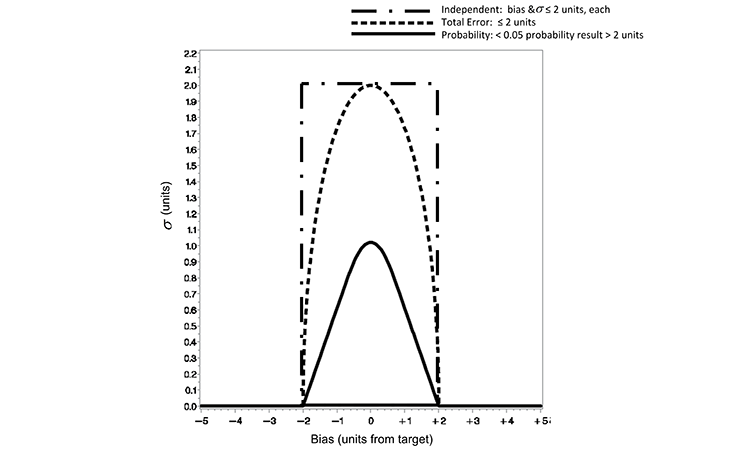
In practice, a quality limit would be defined as a practical limit for the analytical method that may be linked to the product specifications; for the example case provided in this article, a quality limit of two units is defined. The quality metric for each of the three loss functions is defined in Table A. Each of the defined loss functions restricts the range from target to be not more than two units. While all of these approaches are valid and may be applied at the supplier’s discretion, there are practical differences between the approaches.
Figure 1 displays contour plots for the three loss functions defined in Equations 1 to 4. The plots illustrate the relationship, as defined by the functions, of precision (?) and accuracy (distance from target). The parabolic shape of the total error and probability loss functions is also displayed in Figure 1.
“The probability loss is a pragmatic criterion useful for defining the maximum risk of observed results residing farther than a prespecified range.”
Obviously, a method with no bias (zero on the x-axis) can accommodate the largest variability. A method with measurable bias (not zero on the x-axis) must demonstrate reduced variability, decreasing to zero for ever-increasing bias to ensure the same loss limit. This is illustrated for the probability < 0.05 and total error ≤ 2 unit curves in Figure 1. When employing the independent loss approach, which sets separate limits for bias and precision, there is no trade-off between accuracy and precision. The independent loss approach implies that a method may have maximum allowable bias and imprecision simultaneously with no defined joint cost—as seen in the upper left and right corners of the black rectangle.
Characteristics of the loss functions clearly illustrate a difference in the maximum ? (y-axis) allowed for the quality metric limits defined. Defining the total error and independent limits to be ( ? ≤ 2) and (b,s ≤ 2), respectively, allows for a much more liberal limit of variability than that defined by the probability loss quality limit in Figure 1 (p < 0.05 and e = 2). As defined for this example, the total error and independent limits allow an analytical method to produce results with much greater variability than a method that is controlled to the limits defined by the probability loss quality limit.
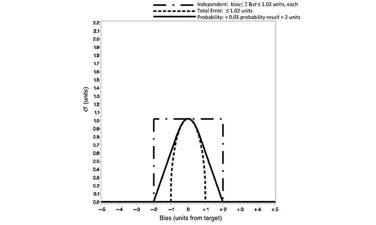
The quality metric criterion defined by the three loss functions is redefined below to account for this disparity in the allowable variability. An equitable comparison can be made by restricting the maximum ? of the total error or independent loss function to equal that of the probability loss function at the zero distance from the target value. By defining the ? in the total error loss function of Equation 1 as the ratio of the allowable range or loss (e.g., e = 2) by an appropriate z-score (1.96 for a 95% two-sided confidence of the normal distribution), the total error and probability loss functions are equivalent at a zero distance from target. Figure 2 displays such a refinement, for which we can now make a viable practical comparison of the risk of test results outside an a priori–defined range.
Based on the Figure 2 normalization, the quality metric limits (for which acceptance is judged) are redefined for each loss function as shown in Table B. The practical difference in the loss functions’ performance can be seen in the risk of making incorrect decisions concerning experimental results. The risk of accepting a subpotent pharmaceutical product lot has been illustrated in previous work with the independent and probability loss functions.5 Demonstrated here is a comparison of the three criteria against the following quality statement: There exists no more than 0.05 probability of a result being > 2 units from the true target content. This is the quality statement defined in the probability loss function of Equation 2 with e = 2 and p = 0.05.
| Loss function quality limits against which a method is to be judged, Case 1: equal maximum allowance from target | |
|---|---|
| Loss function | Quality limit |
| Total error | Total error ≤ 2 units ( ?) |
| Probability | Probability < 0.05 (p) that individual results will reside > 2 units (e) from target (T) |
| Independent | Bias ≤ 2 units (b) and ? ≤ 2 units (s) |
| Loss function quality limits against which a method is to be judged, Case 2: equal maximum σ units at target | |
|---|---|
| Loss function | Quality limit |
| Total error | Total error ≤ 1.02 units ( ?) |
| Probability | Probability < 0.05 (p) that individual results will reside > 2 units (e) from target (T) |
| Independent | Bias ≤ 2 units (b) and ≤ 1.02 units (s) |
Table C compares the three loss functions illustrated in Figure 2 in the ability to demonstrate a pragmatic decision concerning a result. Table C illustrates theoretical analytical bias values in column 1 (true bias [ ?]) ranging from 0 to 2.00, and the maximum variability (maximum allowable sigma [ ?]) solution calculated from each loss function equation (columns 2, 3, and 4). From these two values, the probability of an assay value, assuming normal (true bias, maximum allowable ? ) distribution, residing > 2 units of the true content is then calculated and reported (columns 5, 6, and 7).
The probability loss function restricts the maximum allowable ? to a level commensurate with the labeled bias amounts that maintain a constant probability; column 6 of Table C shows constant 5% probability for all rows (true bias) except for row 6, which shows 0.0% probability for a true bias at the stated limit of 2%. In contrast, both the total error loss function and independent criterion fail to constrain the variability (maximum allowable ?) in a manner that maintains a constant probability; this is demonstrated in columns 5 and 7, respectively.
As illustrated in the example, the independent criterion allows a result to reside > 2 units from the true content a large percentage of the time, for even moderately biased methods (7.8% probability for a bias of 0.5; see column 7, second row in Table C). While smaller acceptance regions could be defined, the basic premise of increased loss (probability results outside defined limits) for methods that deviate from the target remains when using the independent approach for setting limits of accuracy and precision.
The total error loss function restricts the acceptable region (probability of 5%) more greatly than the probability loss function criterion in this illustration. The acceptable distance from the target (true bias) has been reduced to ±1.02 units in Figure 2, where the quality metric is defined by the total error function in this manner. The consequence is evident in column 5 of Table C for a method that incurs a true bias of 0.5 units or greater; the probability observed value more than 2 units from target is 4.8%, 3.5%, and 0% for methods with true biases of 0.5, 0.75, and ≥ 1.02. The total error approach is overly conservative for most pharmaceutical applications when applied in this manner.
In terms of practicality, the probability loss function clearly defines an appropriate quality metric for assessing an analytical method to produce results for which a risk-based decision can be made with a stated level of certainty. A method that meets the probability loss quality criterion in this example can be said to generate results within ±2 units of target at least 95% of the time. Neither the independent nor the total error loss functions make such a pragmatic risk-defined statement. In fact, the independent criterion allows values to be outside the target range of units, more liberally surpassing the stated quality limit of probability not more than 0.05. Using the total error loss function, depending upon how it is defined, could lead to either unnecessarily conservative criteria, as illustrated in Table C, or unnecessarily liberal criteria, as illustrated in Figure 1.
Example
This example illustrates the practical inferences of using the differently defined ATP mentioned in this article. Defining an ATP criterion even prior to the analytical method development process sets a pragmatic minimal target for accuracy and precision that can be assessed periodically throughout the
development of the method prior to verification or validation exercises. This may be achieved through several carefully planned and executed experiments that explore the method accuracy and precision. The following describes one experiment that examines a method’s ability to provide repeatable sample recoveries.
“ATP can be a tool to define a priori quality criteria for results generated by analytical methods.”
Derivation Of Equation 1
It is desirable to obtain values close to a target, T. A loss is experienced when deviations from the nominal target occur irrespective of the direction. The following quadratic loss function achieves this goal, for a random variable of interest, Y.
Loss=E[(Y−T)2]
For a measured value Y with accuracy {E(Y) = µ} and precision {Var(Y) = ?2} the above loss function has the expected value derived below:
E[(Y−T)2]E[(Y−T)(Y−T)]
=E[(Y2−2YT+T2)]
=E(Y2)−2TE(Y)+T2
Note: Var (Y) = E (Y2 ) – [E (Y)]2 = ?2
So, by adding and subtracting [E(Y)]2 to the above, we obtained the following:
E[(Y−T)2]E(Y2)−2TE(Y)+ T2+{[E(Y)]2−[E(Y)]2}
={E(Y2)−[E(Y)]2}+[E(Y)]2 −2TE(Y)+ T2
=σ2+μ2−2Tμ+ T2
=σ2+ (μ−T)2
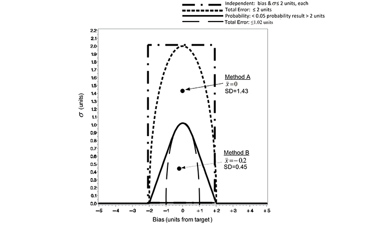
Suppose, as an early development exercise, an analyst executes two methods to assess the sample preparation ease of use. She independently weighs and prepares five composite unit dosage samples from a single batch of material for each of two competing sample preparation techniques (Method A and B) to assess the precision of the methods. Since the true value of samples is not known, the average values (x̅) are determined though separate extraction studies. The average (x̅) from extraction studies and SD of the five composite samples for each method are illustrated against the ATP criteria in Figure 3 and described in the previous section. Because the point representing the (x̅) and SD of Method A falls below the TE ≤ 2 criterion line, Method A would pass this criterion. However, since this point resides well above the TE ≤ 1.02 and the probability criteria (< 5% results > 2 units from target), Method A would fail these criteria. Conversely, Method B passes both the TE ≤ 1.02 and the probability criteria (< 5% results > 2 units from target).
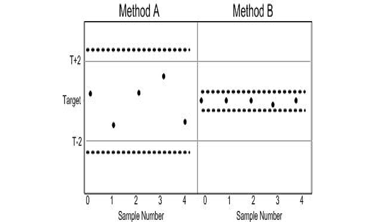
ATP criteria provide a quality metric to further differentiate acceptable methods. Method B expected to elicit samples with TE < 1.02, while Method A can be expected to deliver TE ≤ 2 units. The use of TE as a criterion does not directly identify the consequence of using either Method A or B. The probability loss criterion illustrated does, however. Since the (x̅) and SD of Method B resides below the probability loss criteria in Figure 3, Method B can be expected to produce results that are not more than ±2 units from the target with at least a 95% probability. The pragmatic consequence of accepting either Method A or B as an appropriate measurement system is illustrated in Figure 4.
|
Maximum allowable σ and probability of a reported value > 2 units distance from true amount of pharmaceutical |
||||||
|---|---|---|---|---|---|---|
| Maximum allowable ? (a) | Probability observed value >2 (b) | |||||
| True Bias | Total Error | Probability | Independent | Total Error | Probability | Independent |
| 0.00 | 1.02 | 1.02 | 1.02 | 5.0% | 5.0% | 5.0% |
| 0.50 | 0.89 | 0.90 | 1.02 | 4.8% | 5.0% | 7.8% |
| 0.75 | 0.69 | 0.76 | 1.02 | 3.5% | 5.0% | 11.4% |
| 1.00 | 0.20 | 0.61 | 1.02 | 0.0% | 5.0% | 16.5% |
| 1.50 | 0.00 | 0.30 | 1.02 | 0.0% | 5.0% | 31.2% |
| 2.00 | 0.00 | 0.00 | 1.02 | 0.0% | 0.0% | 50.0% |
(a) Value of σ calculated from each loss function equation given the true bias in the table
(b) Probability: 1−∫2−2ϕ(?:truebias,allowableσ)dy
Both methods may be appropriate in making reliable decisions based upon the samples; the difference in sample-to-sample variability, however, means a greater range in results with the use of Method A and thus a greater risk of decisions concerning the samples residing with the range of target ±2. The evidence is readily seen in a graph of the data as the spread of the samples derived from Method A is much greater than those prepared using Method B. As illustrated in Figure 3, Method B resides within the probability criterion that states not more than 5% of results reside greater than a distance ±2 of the target. This is evident by the inclusion of the 95% confidence bound for individual samples within T ± 2 for Method B in Figure 4.
Conclusion
ATP criteria for judging the quality of results generated by analytical methods have been framed in an optimization paradigm by defining the ATP criteria as a loss function. Two rigorously defined ATP statements to define quality criteria were illustrated in this manner, and compared to historically defined validation criteria. Each ATP statement defined a maximum criterion for deviations of results from a target. One defined this criterion in terms of total error: deviations from the target plus variability. The second defined the criterion as the probability a result resides further from a target than a defined allowance. A comparison of these two criteria and an independently defined criterion of accuracy and precision was made with respect to a decision-based judgment concerning the test results.
The probability loss is a pragmatic criterion useful for defining the maximum risk of observed results residing farther than a prespecified range. Other approaches may be valid and may be applied in line with the acceptable level of risk and at the discretion of the supplier. However, in the case where specifications are based on quality arguments and process capability, the probability loss approach is useful for providing a direct measurement of risk for making incorrect inferences.
Acknowledgments
The authors would like to thank Aili Cheng, Loren Wrisley, and Kim Vukovinsky for their insightful discussions from which this manuscript was inspired.


