Risk-Based Continued Test-Method Performance Verification System

The US FDA and USP have provided guidance for developing, validating, and verifying effective test methods that will deliver quality data.2 ^,3 ^,4 Their guidance calls for continued method performance verification (CMPV) to verify a test method’s performance over its life cycle. At the same time, there has been renewed interest in developing risk-based methods of all types.5 Fortunately, we have concepts, methods, and tools available to build assessment and mitigation of risk into a test-method performance verification system.6

The FDA calls for CMPV.2 ^,3 However, there are three critical risks associated with the long-term use of the method.

• First, the method’s precision in terms of reproducibility and repeatability decreases over time. (Note: Although the pharmaceutical industry often uses the term “reproducibility” to describe between-laboratory variation in measurement results, this article addresses within-laboratory reproducibility, which measures variation due to different analysts, instruments, and other factors at a given laboratory.)
• Second, the method does not meet acceptance limits (specifications).
• Third, management does not pay sufficient attention to method performance.

This article discusses CMPV methods that effectively reduce these critical risks.

Blind Controls to Assess Method Performance Stability over Time

An effective way to assess the long-term stability of a test method is to periodically submit “blind control” samples (also referred to as reference samples) from a common source for analysis along with routine production samples. Blinding the samples ensures that the analyst cannot determine the difference between the production samples and the control samples, and, as Nunnally and McConnell have stated, “There is no better way to understand the true variability of the analytical method.”7

The control samples are typically tested two or three times (depending on the test method) at a given point in time. The sample averages are plotted on a control chart to evaluate the stability (within-lab reproducibility) of the method. The standard deviations of the repeat tests done on the samples are plotted on a control chart to assess the stability of the repeatability of the test method. The deviations of the sample averages from the overall mean measure the within-lab reproducibility of the method. The standard deviation of the test results from the sample mean measures the repeatability of the method.

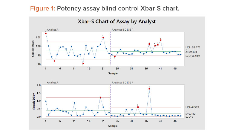
Weitzel and colleagues described a six-year study in which control samples were used to monitor an assay measurement process.8 The blind control samples were drawn from a common master control batch and periodically submitted for lab analysis. Six analysts (A, B, C, D, E, and F) tested the 48 samples in duplicate over the six-year period. See the Appendix for a summary of the results.

Figure 1 shows the control chart for the 48 samples. The first 23 samples were tested by analyst A, and the remaining samples were tested by the other analysts. In Figure 1, we see:

• Analyst A has more within-lab reproducibility issues; several sample averages are outside the control limits.
• There are some within-lab reproducibility issues around samples 37–41; these are principally attributed to analyst C (see the results for analyst C in the Appendix).
• The variation for the other analysts is smaller than that of analyst A.
• The overall average is essentially the same for all analysts.
• Analyst A has larger test-to-test variation (repeatability) than the other analysts.

As we will discuss later, the overall method variation was found to be within the goal of the method.

“Sensitizing rules” are often used in conjunction with control limits to detect nonrandom patterns of variation (level shifts, trends, cycles, and so on), which may not be detected by the control limits.9 These rules increase the sensitivity of the control charts to detect small shifts. One important type of nonrandom variation is out-of-trend results.

Other metrics, such as system suitability test (SST) failures and out-of-limits results, can also be used to assess continued verification. This article focuses on monitoring the results of blind control samples and product stability test results because these test results are widely used and reflect how the test methods are used on a daily basis. SST results have the limitation of measuring only instrument precision, which does not take analyst variation and other sources on variation into account.

Test-Method Stability Metric

The control chart analysis tells us whether we have a measurement stability problem for the particular method being studied. But a lab will have several methods to worry about. Some stability problems are more important than others. This raises the question, “When should we worry about method stability?” The answer is when long-term variation represents more than 20% of the total variation. Note that:

Total variation = Long-term variation (within-lab reproducibility) + short-term variation (repeatability)

The analysis of variance (ANOVA) is used to separate the long-term variance from the short-term variance. ANOVA of the control sample data computes the percent long-term variation, which measures the stability of the test method over time (within-lab reproducibility). Long-term variation variance components less than 30% are generally considered good, with larger values suggesting the method may have within-lab reproducibility issues.10 Collins and associates also discuss the use of long-term variation to assess process stability.11

Control limits may be based on the replicate variation, and this may be an issue when looking for trends. In such a case, the run averages should be subjected to an individuals’ moving average control chart,9 which uses the short-term between-sample variation to calculate the control limits, as discussed by Snee.12

The process stability acceptance criteria for long-term variance are:

• Less than 20% variance indicates measurement process stability is not a problem
• Variance between 20% and 30% suggests that measurement stability may be a problem
• Greater than 30% variance indicates that corrective action may be needed

Figure 2 shows stable (top) and unstable (bottom) measurement processes. The top chart shows a stable process: The long-term variation is 21%, and all points are within the control limits. The variation is random, without trends, shifts, or cycles. This measurement process shows good within-lab reproducibility.

• 2 a b US Food and Drug Administration Center for Drug Evaluation and Research. “Process Validation: General Principles and Practices. Guidance for Industry.” Published January 2011. https://www.fda.gov/regulatory-information/search-fda-guidance-documents/process-validation-general-principles-and-practices
• 3 a b US Food and Drug Administration Center for Biologics Evaluation and Research. “Analytical Procedures and Methods Validation for Drugs and Biologics. Guidance for Industry.” Published July 2015. https://www.fda.gov/regulatory-information/search-fda-guidance-documents/analytical-procedures-and-methods-validation-drugs-and-biologics
• 4USP Validation and Verification Expert Panel. “Proposed New USP General Chapter: The Analytical Procedure Lifecycle <1220>.” Pharmacopeial Forum 43, no. 1 (2017).
• 5International Council for Harmonisation of Technical Requirements for Pharmaceuticals for Human Use. “ICH Guideline Q9 on Quality Risk Management.” European Medicines Agency website. Published 2005. https://www.ema.europa.eu/en/documents/scientific-guideline/international-conference-harmonisation-technical-requirements-registration-pharmaceuticals-human-use_en-3.pdf
• 6Snee, R. D. “Risk-Based Test Method Development, Validation and Life Cycle,” American Pharmaceutical Review, July–August 2019, 64–67.
• 7Nunnally, B. K., and J. S. McConnell. Six Sigma in the Pharmaceutical Industry: Understanding, Reducing, and Controlling Variation in Pharmaceuticals and Biologics. Boca Raton, FL: CRC Press, 2007.
• 8Weitzel, J., R. A. Forbes, and R. D. Snee. “Use of the Analytical Target Profile in the Lifecycle of an Analytical Procedure: With an Example for an HPLC Procedure.” Journal of Validation Technology 20, no. 4 (2015).
• 9 a b Montgomery, D. C. Introduction to Statistical Quality Control, 7th ed. New York: Wiley, 2013.
• 10Snee, R. D., and R. W. Hoerl. “Going on Feel: Monitor and Improve Process Stability to Make Customers Happy.” Quality Progress May 2012, 39–41.
• 11Collins, J., N. Sayeed-Desta, A. B. Pazhayattil, and C. Doshi. “A Novel Metric for Continuous Improvement during Stage Three.” BioPharm International 30, no. 6 (2017): 32–35.
• 12Snee, R. D. “Reducing False Out-of-Control Signals.” Pharma Technology 2014 supplement no. 2 (August 2014): 47–49.

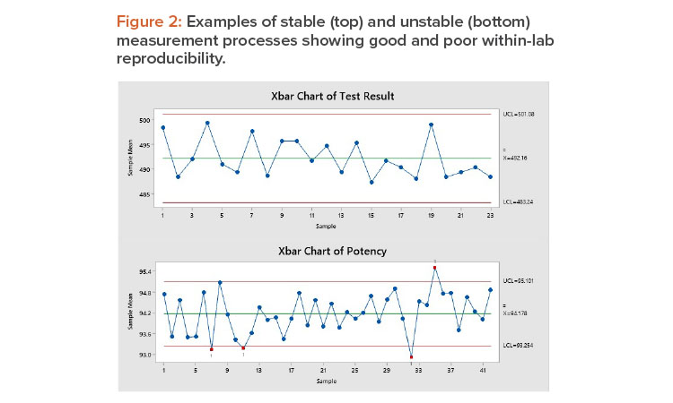
The bottom control chart shows an unstable measurement process: Five of the sample averages are outside the control limits, and the long-term variation is 58%, well above the 30% threshold for corrective action. This measurement process has poor within-lab reproducibility.

Control limits may be based on the replicate variation, and this may be an issue when looking for trends.

The process stability acceptance criteria stated previously are recommendations that may be revised to suit specific applications. Also, when the criteria indicate that within-lab reproducibility and/or the total measurement variability may be a concern, one should look at how the variation in the test results compares to the acceptable limits (specifications) for the measurement method. This issue is addressed later, in the discussion of test-method performance capability indices.

ANOVA is used to calculate the portion of variation that is attributable to measurement repeatability and within-lab reproducibility.9 Table 1 shows the ANOVA of the test results for analyst A in the potency assay study as well as the associated variance components. In Table 1, we see that the sample-to-sample variation (within-lab reproducibility) is statistically significant (P = 0.000). Within-lab reproducibility accounts for approximately 70% of the total variation in analyst A’s test results, with the remaining 30% being due to repeatability variation.

Table 2 summarizes variance component statistics for all analysts, analyst A, and analysts B, C, D, E, and F. Here we see that variation for analysts B, C, D, E, and F is 40% of the total, a little above the 30% guideline. The good news is that the total variance goal of 1.0 is met by analyst A as well as the other analysts.8 So, although within-lab reproducibility may be high for this method, the results are within the goal for the method, which is relatively tight (relative standard deviation = 1%).

• 9
• 8

Product Stability Data to Assess Method Performance

The use of blind controls to assess measurement stability may have drawbacks. The first concern is that resources are required to maintain the control sample and insert the blind controls with the routine production samples. Furthermore, try as you might to keep the controls blinded, there is a risk that analysts will identify the blind controls and their purpose.

Whereas blind controls are used to routinely test a common product over time and observe the variation in the test results, Ermer and colleagues have noted that product stability data are another source of such data.13 In a product stability study, at least one batch of the product is typically tested using a common test method at various time points to assess the stability of the product.

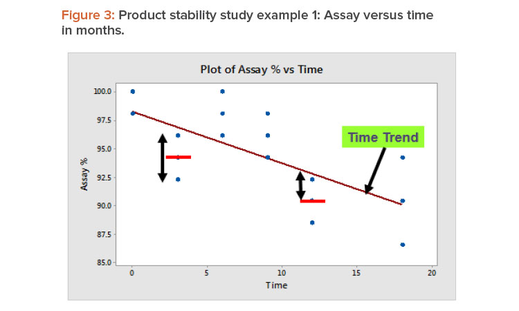
In product stability studies, after the time trend has been accounted for, the variation remaining is due to the test method’s repeatability and with-in-lab reproducibility. Figure 3 illustrates this by showing the relation between assay % and time measured in months for example 1 from Table 3. Repeatability is the variation around the sample mean, as illustrated by the data at three months. Within-lab reproducibility is the variation between the sample mean and the trend line, which is illustrated by the 12-month data.

Table 4 presents the ANOVA for example 1 (Table 3) as well as the associated variance components. In this case, reproduciblity accounts for 45% of the total measuremeent variation. The lack-of-fit P value (0.042) indicates that within-lab reproducibility is statistically significant.

Product stability study example 2 data show a more complicated data set (Table 5). Here, five lots have been put on a stability test. Duplicate test results were made at each of eight time points (0, 3, 6, 9, 12, 18, 24, and 36 months). Scatterplots of assay results versus time (not shown) identified linear trends for the different lots. The overall adjusted R2 equals 80% for these relationships. An examination of these plots shows several instances where the duplicate points are both above and below the trend line, indicating within-lab reproducibility variation. Variation between pairs of duplicate results reflects the repeatability of the method.

The ANOVA and variance components (Table 6) show that within-lab reproducibility accounts for 34% of the total measurement variation, which is above the stability acceptance criteria (<30%) discussed earlier. The ANOVA model allows for the slopes of the trend line to vary between lots. The residual variation is due to the test-method variation: within-lab reproducibility (lack-of-fit) and repeatability (replicates). The lack-of-fit P value (0.017) indicates that within-lab reproducibility is statistically significant, although it is not large as measured by the criteria for long-term variation criteria (acceptable <30%).

Assessing Test Method Capability

Measurement systems typically define acceptance criteria in terms of a goal standard deviation or upper and lower limits (USL, LSL), which are called “specifications” here.

The measurement system’s performance can be assessed using the process performance capability index (Ppk):

Ppk = A/B
where A = minimum (USL – Average, Average – LSL)
and B = 3 (standard deviation).

A generally accepted minimum value for Ppk is 1.33, which is consistent with 0.006% of the test results being outside of the specifications. This calculation assumes that the measurement process is stable and the measurement variation follows a normal distribution. Process performance capability indices are applicable to measurement processes because measurement is a process.

Table 7 summarizes the Ppk index for the potency test method data (Figure 1, Tables 1 and 2). As expected, the Ppk value for analysts B, C, D, E, and F (Ppk = 1.57; 95% confidence limits 1.25–1.90) is higher than that for analyst A (Ppk = 0.98; 95% confidence limits 0.75–1.20). These results were confirmed when the test results were compared to specifications (target measurement uncertainty = 90–110) and the Ppk values and their 95% confidence limits were examined.

The capability analysis is useful because it compares the measurement variation to the specification limits (acceptance criteria) of the test method. The frequency of out-of-specification results is done as part of the analysis.

One of the outputs of the analytical target profile is a set of acceptance limits that are the same as specifications for the output of the measurement.4 As noted previously, the acceptance limits in this case were 90–110.

The sample size used to estimate the Ppk capability index is a critical consideration. Capability indices require larger sample sizes than might be expected. From a practical perspective, the sample should contain data that represent the total range of product values that the method is expected to measure. For example, if the total range of values for a particular measurement typically seen for a product is 90–110 and the data set contains values that range from 92 to 98, the sample is not representative of the total range of values.

From a statistical perspective, capability indices are highly variable when estimated from small samples. Studies have shown that, at a bare minimum, the sample size should be larger than 30–60, with the preferred sample size being greater than 60–90.14 Additional data on the uncertainty associated with the capability indices can be found in reference 14. That analysis shows that the length of the confidence intervals is wide, even for a sample size of 60.

Reporting the lower confidence limit for the performance capability index is a conservative strategy that takes sample size into account. For example, consider a sample of size 30, for which Ppk equals 1.30. This is close to the preferred minimum of 1.33, but the confidence limits are wide (1.02–1.76). By reporting ”performance capability index = 1.02 (lower 95% confidence limit),” we have reported a performance capability index that has taken the limited sample size into account. Of course, the lower confidence limit can be increased by increasing the sample size.

Risk of Lack of Management Attention

We often hear the comment that test methods receive insufficient attention from management. If management put test methods higher on their priority list, more resources would be made available to support measurement systems, which would in turn increase the chances that better measurement systems will emerge. One way to get management attention for test methods is to include method performance data as part of the management review of production data. Such an approach is shown in Figure 4.15 This strategy seems reasonable because the test methods are used to produce the production data.

• 13Ermer, J., C. Arth, P. De Raeve, D. Dill, et al. “Precision from Drug Stability Studies: Investigation of Reliable Repeatability and Intermediate Precision of HPLC Assay Procedures.” Journal of Pharmaceutical and Biomedical Analysis 38 (2005): 653–63.
• 4
• 14American Society for Quality Chemical and Processes Division. Quality Assurance for the Process Industries: A Manual of Best Practices, 2nd ed. Milwaukee, WI: ASQ Quality Press, 1999.
• 15Snee, R. D. “Management Holds the Key to Continued Process Verification.” Pharmaceutical Manufacturing January/February 2015: 33–35. https://www.pharmamanufacturing.com/articles/2015/management-holds-the-key-to-continued-process-verification

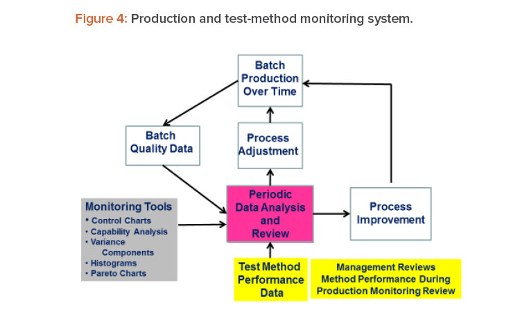
Figure 4 is a schematic of a system that links method performance data with the process, its data and analysis, management review, process adjustment, and process improvement. Process adjustments are changes made to bring the process back to target and/or within specifications. Process improvements are process changes made to correct problems in process performance. Process improvements typically result from team-led process improvement projects using an improvement framework such as define, measure, analyze, and improve and control (DMAIC).16

This results in a system for CMPV as well as continued process verification, as called for in the FDA guidance.2 ^,3 When we add test-method performance data to the system, we achieve CMPV as recommended in the USP guidance.4 Although this article focused on the monitoring of test-method measurements, out-of-specification, out-of-trend, and system-suitability-failure events can also be added to the metrics monitored.

I refer to management review as the “secret sauce.” Requiring periodic management review of measurement systems is a giant step forward toward the long-term sustainability of effective measurement systems. Management review is a “team sport” done by different management teams at different times. These teams include process operators (daily/hourly), area management (weekly), site management (monthly), and business management (quarterly). The management review plan should be devised to suit the needs of the business. Test-method performance would typically be assessed less frequently (e.g., monthly or quarterly) than process performance. The schedule selected will, of course, depend on the specific needs of the organization involved.

Trust but Verify

The admonishment to “trust but verify” applies to the monitoring of test methods. The tools described in this article provide an effective check on test-method stability and capability, and they reduce risk. The use of blind control samples is effective. The use of product stability data also works; this method is a broader and more robust verification check and reduces cost. Commercially available software can be used to carry out the calculations and analyses required for the proposed approaches. The proposed systems approach with integrated management review helps maintain the stability of test methods over time. This results in reduced risk of poor manufacturing process performance and defective pharmaceuticals reaching patients.

• 16Snee, R. D., and R. W. Hoerl. Leading Six Sigma: A Guide Based on Experience with General Electric and Other Six Sigma Companies. New York: FT Prentice Hall, 2003.
• 2
• 3
• 4