Embrace Special Cause Variation During Continued Process Verification (CPV)

Understanding the fundamental assumption of independence (and the violation thereof) enables an appropriate response to control chart trend rule violations and challenges us to think differently about special cause variation in control charts.
To align with the 2011 US Food and Drug Administration (FDA) guidance on process validation, actions must be taken during the continued process verification (CPV) stage so that “[o] ngoing assurance is gained during routine production that the process remains in a state of control.”1 Process monitoring during this stage provides valuable information that can be used to address process problems and identify opportunities for improvement. Successful implementation of CPV requires not only that decisions and actions be aligned with these goals; the use of statistical tools such as control charts must also be understood within the context of pharmaceutical/biologics manufacture and a risk-based approach to lifecycle process validation.
Discussion
It is common practice to use Shewart control charts to monitor process behavior during the CPV stage. Quite often manufacturers apply a selection of the Western Electric or Nelson rules* to their control charts.2 ,3 These rules were designed to signal significant process change and to justify action, often in real time, to address the change in process behavior.
Often not incorporated into the design and interpretation of these control charts, however, is the influence of the most important assumption underlying conventional interpretation: independent observations.4 When observations are independent, variation is a result of random sources; the output of batch #1 is no more similar to batch #2 than it is to batch #25. Because this assumption is rarely met for pharmaceutical quality attributes, adaptation of typical control chart interpretation is critical; otherwise, CPV programs can be designed that not only misguide and waste resources, but actually hinder CPV goals.
Why is understanding this assumption so critical to a successful CPV program? Reach for almost any Lean Six Sigma reference to process control and you will find variability described as either “common cause,” due to typical, random sources of variability, or “special cause,” which reflects unexpected variability that is likely the result of a process change. Further description of the two types typically assigns an assessment of process control. Specifically, a process displaying only common cause variation is often said to be “in control” or “stable and predictable.” Special cause variation, in contrast, is generally described as unexpected or unnatural variation, and indicates that the process may be “unstable and unpredictable” or “out of control.”5 ,6 ,7
The immediate translation of a statistical signal to potential loss of process control is valid only if the fundamental assumption of independence is met.
When a process is in a state of control and sources of variability have random influence across time, points on the control chart should have a random pattern.4 , 8 Evidence of special cause variation can be an unexpected event, such as a single point outside of a control limit or a pattern not expected by random chance. In commonly used statistical software packages, such events can be associated with the Nelson rules, and identified on a control chart as a red symbol and a number identifying the specific pattern, commonly referred to as a statistical signal. This special cause designation is often associated with a call for action or investigation into the process to bring it back to a state of control. Thus, “red” is viewed as a problem. Some references are more extreme, stating that special causes must be eliminated before the control chart can be used as a monitoring tool.8
It is critical to understand, however, that the immediate translation of a statistical signal to potential loss of process control is valid only if the fundamental assumption of independence is met. And in the usual manufacture of pharmaceutical and biological products, nonindependence is the norm, since typical sources of variability (raw materials, equipment, lab factors, etc.) are not used randomly. They meet the “typical” and “expected,” but not “random” criteria of the common cause variability definition.
In this scenario, patterns of variability that result from the nonrandom use of these typical sources may be identified as special cause variation. Practically speaking, this is a different situation than special cause variation that results from a true process upset, such as error in addition of raw materials. In the realm of non-independence, overreaction can occur when all special cause notations are automatically perceived as reflections of a process that is out of control.
* To distinguish between natural and unnatural variation, Western Electric expanded on the three standard error decision rules of Walter Shewhart. Based on these decision rules, Lloyd Nelson later formulated a set of tests for assignable causes.
- 1US Food and Drug Administration. Guidance for Industry. “Process Validation: General Principles and Practices.” Revision 1. January 2011. http://www.fda.gov/downloads/Drugs/.../Guidances/UCM070336.pdf
- 2Western Electric Co., Inc. Statistical Quality Control Handbook. Easton, Pennsylvania: Mack Printing Company, 1956.
- 3Nelson, Lloyd S. “Technical Aids.” Journal of Quality Technology 16, no. 4 (October 1984).
- 4 a b Montgomery, Douglas C. Introduction to Statistical Quality Control, 7th ed. John Wiley & Sons, Inc., 2013.
- 5George, Michael L., et al. The Lean Six Sigma Pocket Toolbook, McGraw-Hill, 2005.
- 6Wedgewood, Ian D. Lean Sigma: A Practitioner’s Guide, Prentice Hall, 2007.
- 7Brue, Greg. Six Sigma for Managers, McGraw-Hill, 2002.
- 8 a b Six Sigma Academy. The Black Belt Memory Jogger, 1st edition, GOAL/QPC, 2002.
If non-independence precludes the conventional interpretation of trend rules and special cause variation,4 ,5 does that mean basic control charts can’t be used? Certainly not. These tools, in their simplest forms, are very powerful, even in the presence of non-independence. The nonrandom use of variability sources (such as different raw material lots) is not the problem. The problem results when control chart interpretation is not appropriately modified from the classical statistical process control (SPC) paradigm in which independence is assumed.
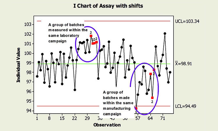
When common cause sources of variability are not used randomly across time, “unlikely” patterns are really not so unlikely. For instance, the pattern of nine points on the same side of the control chart centerline can be expected. These patterns do not necessarily indicate that the process is out of control; it is often a reflection of the process as designed. The absence of statistical signals cannot be required to claim a state of control. Because of non-independence, the “state of control” may include results identified as special cause variation, as shown in Figure 1.
The figure shows two shifts in the data, one representing a group of batches measured in the same laboratory campaign, and another produced during the same manufacturing campaign. The observed behavior is not inherently unexpected; the process is not necessarily “out of control,” in the sense that the shifts in mean forecast instability and risk. The shifts may in fact be expected, since batches within the same laboratory and manufacturing campaign share common sources of variability that are quite likely different from the other campaigns represented. Even the point below the lower control limit is a potential artifact of non-independence. (See the discussion preceding the conclusion.)
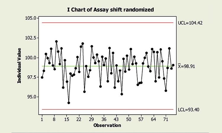
Figure 2 is a chart of the same data in random order. Randomizing results reflects what could be expected if the common cause variables that influence individual campaigns were experienced randomly across time. Not surprisingly, no special cause variation is identified. Note, too, that the true process performance in Figure 2 is no better than that of Figure 1. Process performance and control cannot be measured by the amount of “red.” The charts could be interpreted incorrectly if the underlying data structure—and its effects on chart interpretation—were not understood.
Given this context, the appropriate response to this variation is not as straightforward as a simple textbook case, where a red symbol on a control chart becomes a call for action. Nor are the patterns and resulting signals in Figure 1 false alarms in the statistical sense; they do indicate performance that is statistically unexpected relative to overall performance. Thus, they can provide valuable information regarding the sources of variability, directly enabling the CPV goals of ongoing quality assurance and continual improvement.
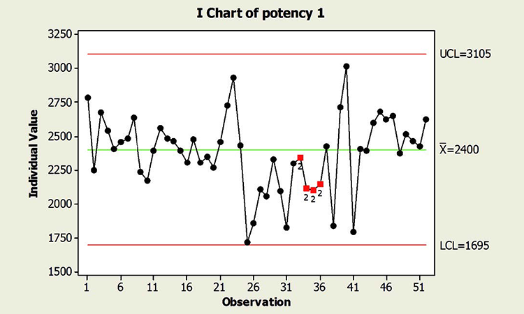
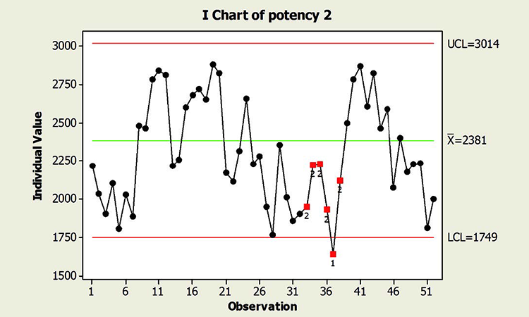
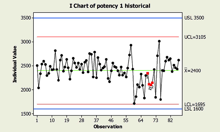
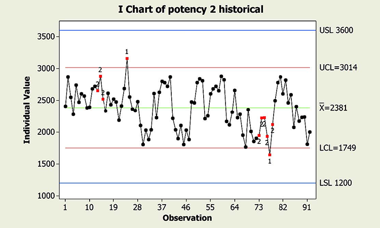
When textbook statistical interpretation of signals is not valid, a risk-based approach can define the urgency and appropriate reaction to special cause variability. Consider the following pair of charts: In each case, a shift in the mean is identified with a red number 2 following 9 points in a row on the same side of the mean. The magnitude of the shift relative to overall performance is about the same. But should reaction to these patterns also be the same?
In a presentation at the 2015 ISPE Statistician Forum on process validation, a member of the FDA Center for Drug Evaluation and Research, Office of Pharmaceutical Quality, noted that “…all signals are not created equally” and “… magnitude of the response depends on the severity of the signal …”9 In this hypothetical situation, how might that advice be interpreted? Both figures reflect the same attribute (potency), and it is likely that potency would be rated as a high severity attribute. Does that mean that every signal must be investigated, and to the same level? What additional information might be useful to define the severity of the signal and an appropriate response in each scenario?
Consider the charts in Figure 4, which include more historical data prior to the shift, and specification limits (blue lines). This additional information is used to assess: 1) if the pattern is truly unexpected, and 2) risk.
- 9Viehmann, Alex. “Process Monitoring Expectations and Establishing Acceptance Criteria.” Presented at the ISPE Statistician Forum, Silver Spring, MD, 14–15 April 2015.
Using control charts in CPV requires a mindset change from typical application and interpretation within the SPC paradigm.
In addition, because this type of behavior has not been observed in the past, this shift is unexpected. And although the process has returned to normal behavior, we cannot know whether the factor that caused the shift will occur again; if it does, the risk of results outside specification is clearly apparent. In this situation, therefore, immediate attention is warranted.
This contrasts with the situation shown in the Potency 2 chart. Not only is the process trending well within specifications, shifts similar to the most recent one have been observed historically. Note that like the shift in assay in Figure 1, patterns identified in the Potency 2 data could indeed provide valuable information about sources of variability, and opportunity for continual improvement, thereby enabling a primary goal of CPV. The urgency for investigation, however, would not rise to the level warranted for the Potency 1 situation.
While process knowledge may certainly be gained through the evaluation of signals, the requirement that they be investigated regardless of the risk to patient and business can result in substantial, misdirected resources. Ultimately, this lack of prioritization serves neither the patient nor the business. Akin to the previous example, some manufacturers have designed decision trees or matrices to incorporate a risk-based approach to statistical signals in control charts and ensure an appropriate level of attention is given to observed signals.
Examples of decision rules include:
- Process capability (e.g., using process performance index)
- Distance of signal from specification
- Distance of signal from mean
- Number of batches affected
- Historical patterns of variability
Signal response is commensurate with the risk and opportunity identified considering those multiple elements, and can vary from a simple acknowledgment at the lowest level to a formal investigation documented within the quality system. The BioPhorum Operations Group CPV and Informatics Team formulated one such risk-based approach to signals, published in the January-February 2017 issue of this magazine.10
Fearing unnecessary attention to signals and knowing that they are expected, some manufacturers choose to remove these signals from their charts. If the context were real-time SPC requiring rapid process-adjustment decisions, the number of signals may indeed pose a problem. But this does not pose the same risk in CPV, where immediate adjustments or decisions are not typically sought. And if the business process defines a risk-based approach to signals, overanalysis and/or overreaction should not occur.
When special cause variation triggers an appropriate risk-based response, the resulting visible patterns can help achieve CPV goals.
Questionable effectiveness is another reason some manufacturers choose to omit signals. For instance, specific statistical requirements can result in the situation of a shift that is detectable by a keen eye, but does not trigger a signal. The logic for omission continues: If signals are not triggered for all shifts and they can be misinterpreted as a lack of control, why use them at all? Indeed, careful review of charts for excursions and patterns by a process subject matter expert can be more effective than simple reliance on statistical signals. This careful review does not always exist, however, and even when it does the pattern of color from signals can aid interpretation. This is particularly true in early stages of process understanding, due either to the age of the product or the age of the CPV program.
There may indeed be cases where it’s reasonable to omit specific signals, as they provide little benefit or may even be detrimental. This decision should be considered carefully, however, by assessing what knowledge about variability might be forfeited, and recognizing that the biggest value of the charts can be the pattern they reveal.11 If signals are viewed negatively due to inadequate training of users and reviewers, cumbersome reporting, or overreaction, more benefit may be realized by addressing these deficiencies than by widespread omission.
An additional note regarding both examples: These charts have “Shewhart” control limits derived from the average moving range, thus they reflect short-term standard deviation. In the context of nonrandom variability sources, this estimate tends to be less than the longer-term estimate computed by the typical standard deviation formulation of a sample. For this reason, Shewhart limits may be too narrow to bracket expected total variability, and more values may be expected to be outside the limits compared to the number expected if sources of variability are truly random. Hence, some manufacturers choose to derive limits based on the longer-term estimate of standard deviation. Others maintain the short-term estimate, and recognize this feature in their risk-based response to statistical signals.
CONCLUSION
Using control charts in CPV requires a mindset change from typical application and interpretation within the SPC paradigm. Indeed, while both paradigms utilize control charts, their intended use and assumed data structure are not the same. Thus, it should be expected that interpretation also differs. Because the fundamental assumption of independence integral to conventional SPC is not met in typical pharmaceutical or biopharmaceutical manufacture, response to variation identified as special cause is unfortunately not a simple application of statistical rules and common definitions.. Ignoring the influence of this assumption and imposing actions as if it had been in fact met is not only statistically inappropriate, it can result in wasted resources, improper focus, lost opportunities, and frustrated employees. None of these outcomes serve either the business or the patient. And while omitting the identification of “expected” special cause variation to avoid too many signals might be important in the context of real time SPC, it can inhibit the CPV goal of continued understanding of process variability.
Control chart interpretation within the context of CPV requires a combination of process knowledge, adequate statistical understanding, and a business process that incorporates them into a risk-based decision framework. When special cause variation triggers an appropriate risk-based response, the resulting visible patterns can be embraced to help achieve the goals of CPV.
Instead of dreading statistical signals in control charts, a new appreciation can be acquired where “red is the new black.”